CROPWAT Training: A Step-by-Step Guide to Estimating Crop Water Requirements
In the past, estimating the water needs of crops like corn was a challenging task due to the lack of precise tools and data integration methods. This often led to inefficient water use, over-irrigation, or under-irrigation, resulting in reduced crop yields and wasted resources.
Considering that more than 45% of the world’s corn is produced in the United States, can you imagine an exact number for the daily water requirement of this vital crop? In the past, estimating the water needs of crops like corn was a challenging task due to the lack of precise tools and data integration methods. This often led to inefficient water use, over-irrigation, or under-irrigation, resulting in reduced crop yields and wasted resources. However, advancements in agricultural technology, such as the development of software like CROPWAT, have revolutionized this process. By incorporating climatic, soil, and crop-specific data, CROPWAT allows for accurate and straightforward calculation of crop water requirements. Even for crops like corn that require a lot of water, farmers and researchers can now optimize irrigation schedules, cut down on water waste, and increase productivity with the help of tools like these, guaranteeing sustainable farming practices.
In order to manage water resources in irrigation and drainage plans, it is necessary to estimate water requirements. To determine the water requirement, the evaporation and transpiration potential of the reference plant (ET0) should be estimated. To estimate the amount of evaporation and transpiration, there are different methods such as FAO-Penman-Monteith (FAO, Chapter: FAO- Penman- Monteith equation), the Blaney-Criddle (FAO, Chapter3:Crop Water Needs) and the Hargreaves method (Hargreaves and Samani, 1985).
In this project, we are going to obtain the water requirement of the corn plant using the data of 1974 to 2024. We estimate the crop water requirement using the CROPWAT software. This software uses the Penman-Monteith method. Therefore, it is time to start the training of determining the crop water requirement with this software.
1. Designing the System by CROPWAT
In this article, we aim to estimate the water requirements of corn in Overland Park, Kansas, United States, by utilizing detailed climatic, soil, and crop data specific to the region. The process involves analyzing local environmental conditions, such as temperature, rainfall, and evapotranspiration rates, and applying advanced methods to calculate crop water demands.
Additionally, the article provides a step-by-step explanation of the methodology, making it a comprehensive guide for users wishing to understand or replicate the process in similar regions. The study uses CROPWAT to ensure accurate and reliable results, offering insights into irrigation needs and sustainable water management practices for corn cultivation in Overland Park.
1.1. Software
CROPWAT 8.0, which was developed by the Land and Water Development Division of FAO, is a decision-support tool designed to calculate crop water and irrigation requirements that uses soil, climate, and crop data. The software facilitates the development of irrigation schedules under various management scenarios and estimates water supply for diverse cropping patterns. It also evaluates irrigation practices and estimates crop performance in both rainfed and irrigated conditions. CROPWAT uses methodologies outlined in FAO's Irrigation and Drainage Series No. 56 ("Crop Evapotranspiration") and No. 33 ("Yield Response to Water").
The program incorporates climatic data from over 5,000 global stations via the CLIMWAT database, ensuring usability even when local data is unavailable. Users can input monthly, decade (10-day intervals), or daily data for precise calculations of reference evapotranspiration (ET0) and crop water requirements. With features like interactive irrigation schedules, daily soil-water balance outputs, and graphical presentations, CROPWAT provides a user-friendly platform for managing irrigation. It supports multiple languages and is compatible with various Windows platforms, making it a versatile tool for agricultural water management.
Fig. 1. The CROPWAT software interface for Windows, a tool for estimating crop water requirements.
The CROPWAT software requires four steps in which the user should enter the data. The CROPWAT software tabs are introduced and explained in sections Basic requirements for design (1.2) and inputs (1.3). After entering the required inputs, the Cropwat software displays outputs. These outputs are explained in Section Output (1.3). Notice that in each step the changes should be saved before proceeding to the next section.
1.1. Study Area
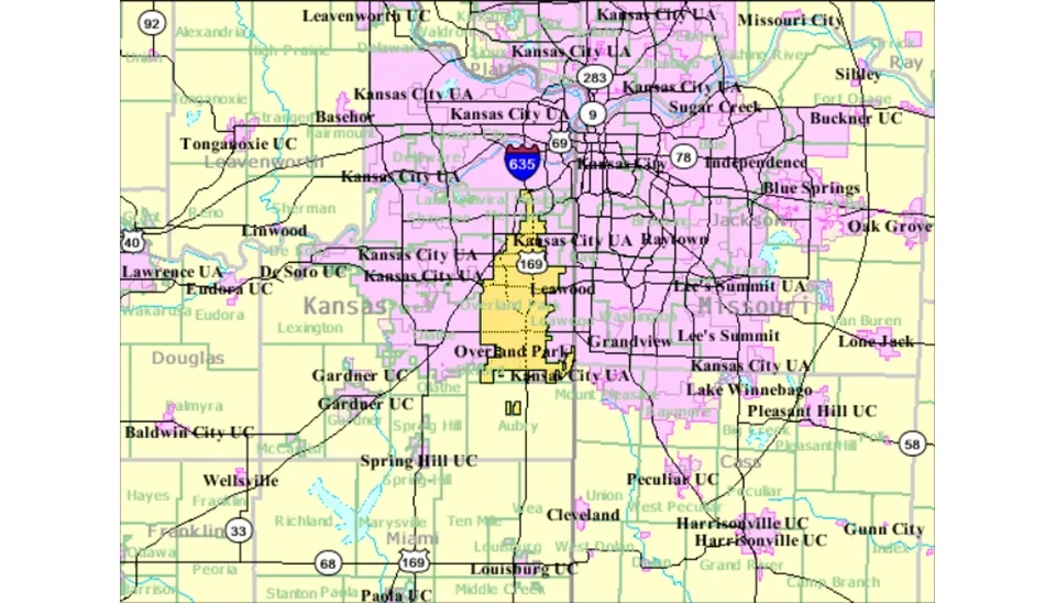
Overland Park, located in northeastern Kansas, USA, is characterized by a humid continental climate that influences the water requirements for crops, particularly corn. You can see the location of Overland Park in the United States of America in figure 2.
Fig. 2. Overland Park location in the State of Kansas
Summers in Overland Park are typically warm and humid, with average temperatures between 25-30°C (77-86°F) during the peak growing season, which coincides with the primary period of water demand for corn. These warm temperatures contribute to high rates of evapotranspiration, increasing the need for consistent moisture to sustain crop growth. Winters in Overland Park are cold, with temperatures often dropping below freezing; however, these conditions generally fall outside the corn-growing season (figure 3).
Fig. 3. Typical summer and winter weather conditions in Overland Park, Kansas.
Precipitation in Overland Park is relatively evenly spread throughout the year, but it reaches its highest levels during late spring and summer, aligning well with the period when crops like corn requires the most water. The annual average rainfall is approximately 920 mm (36 inches), providing a natural source of water; however, dry spells are common, particularly during late summer, which may necessitate supplemental irrigation to maintain optimal growth. Additionally, high summer humidity levels, along with wind, can impact evapotranspiration rates, creating variability in the crop’s water needs. Understanding the specific climate dynamics in Overland Park is essential for developing effective irrigation strategies and ensuring sustainable water use in corn production within this region (weatherspark).
1.2. Basic requirements for design
In the CROPWAT software we have 8 main tabs, four of them are related to input tabs that we use the meteorological data and selected crop information, as well as the soil data. Then the CROPWAT software presents outputs in different windows so that we can use this information to estimate the crop water requirements for corn plants.
1.3. Inputs
This software consists of four input tabs. The first is Climate/ET0, the second is rain, the third is crop, and the last is soil data. In the following, each of them will be discussed. Let us introduce the first tab named Climate/ET0 as the first input data requirement.
1.3.1. Climate/ET0
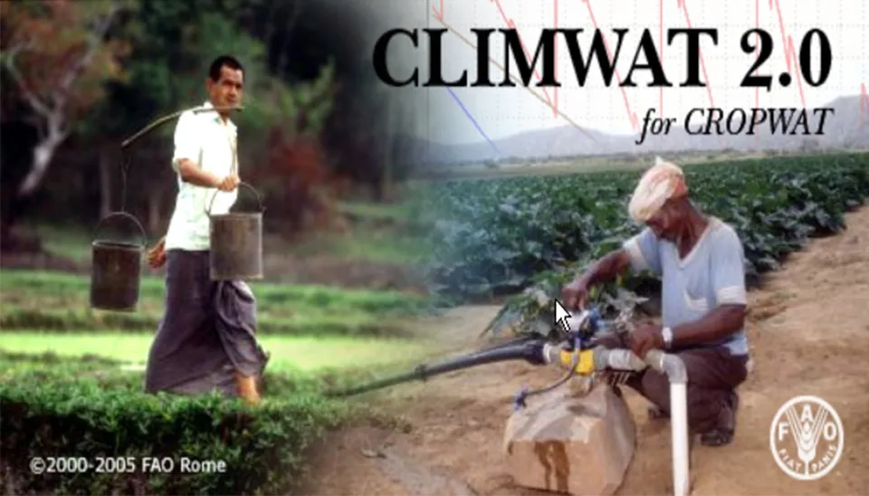
The first section in the CROPWAT software is “Climate/ET0. For this section, we can use the meteorological data from weather sites. Additionally, you can download and install the CLIMWAT from the FAO website (Figure 4). The CLIMWAT is the climate database, which is used with CROPWAT and it provides CROPWAT with meteorological data from more than 5000 weather stations worldwide, and with this help, it can be used to estimate crop water requirements, irrigation supply, and irrigation scheduling. Therefore, when you do not have any data, using the CLIMWAT software seems like a beneficial option for users (CLIMWAT).
Fig. 4. The CLIMWAT Software interface
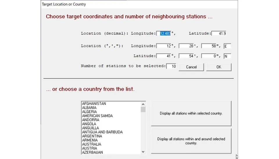
The FAO states that the CLIMWAT software in its database has the long-term monthly mean values of the following climate parameters required for the calculation of potential evapotranspiration according to the Penman-Monteith method: mean daily maximum temperature, mean daily minimum temperature, mean relative humidity, mean wind speed, mean sunshine hours or solar radiation, total and effective monthly precipitation. All variables, except potential evapotranspiration, are direct observations or transformed observations (FAO-Land & Water). After installing this software, you can see the target location or country. In this window, you have ways to receive station information. You can see the figure 5. In the first way, by entering the latitude and longitude, you will be provided with the information from the nearest synoptic station. In the second method, you can select the country in question, and all the stations whose data is in this database will be displayed to you (see figure 5).
Fig. 5. Target Location or Country within The CLIMWAT Software
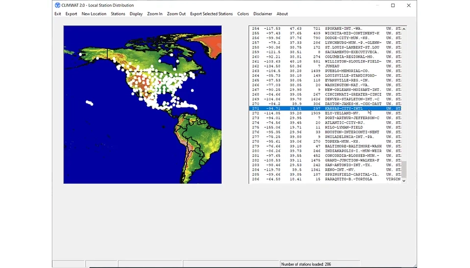
After selecting one of those methods mentioned, you can select the station you want to view using the map, locations on it, or from the list on the left. Then, you can get the station data from the Export Selected Station option (Fig. 6).
Fig. 6. Local Station Distribution in The CLIMWAT Software
Finally, the CROPWAT software allows you to import two specific file types, .pen and .cli, into the climate and rain sections, respectively, to run the model using this data. The .pen file typically contains climatic data, such as temperature, humidity, and wind speed for calculation the Penman-Monteith reference evapotranspiration (ET0) values, while the .cli file stores the Monthly Rainfall data and calculates the Effective rain in mm. These files enable users to input detailed, pre-prepared datasets to enhance the accuracy of the calculations and tailor the model to specific conditions. In this project, for data required, we use the weather website that is mentioned in Section (1.1). In the “Climate/ET0” section, the first part is shown in figure 7.
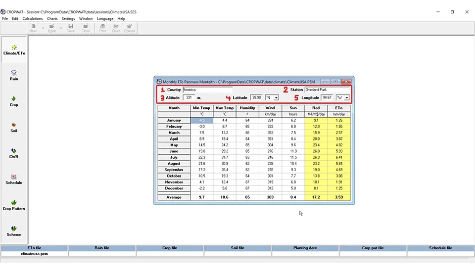
Fig. 7. Basic Information in the ClimateET0 Window.
The red box at the top of the window contains the following:
Country: United States of America
Station: Overland Park
Altitude: 331m (1086 ft)
Latitude: 38ᐤ 58’ 54’’ N
Longitude: 94ᐤ 40’ 16’’ W
As you can see, in this project we considered the Country of the United States of America and Overland Park station. The Altitude above sea level in Overland Park is 331 meters (1086 feet). Latitude is degrees north or south, which is equal to 38 degrees, 58 minutes, and 54 seconds for Overland Park. Also, Longitude is degrees east or west, which for Overland Park is 94 degrees, 40 minutes, and 16 seconds. It is necessary to convert the minutes and seconds into degrees for use in CROPWAT software, so the latitude of Overland Park is 38.98 degrees north and the longitude of Overland Park is 94.67 degrees west. The second part in climate/ET0 shown in figure 8:
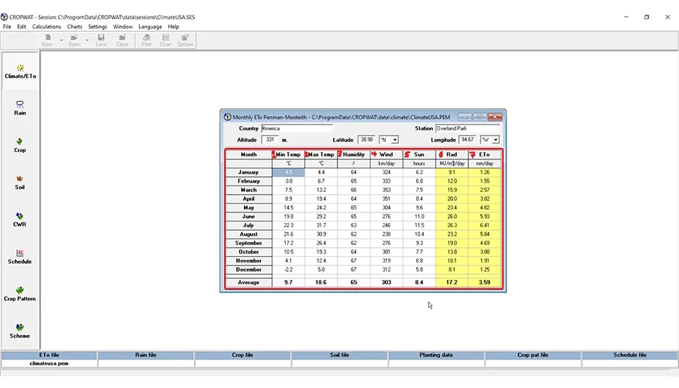
Fig. 8. Monthly Meteorological Data and Monthly ET0 (Penman-Monteith) in the Cropwat Software
According to Figure 8, other required data are:
Min Temp
Max Temp
Humidity
Wind
Sun
Which are expressed as monthly averages in such a way that Average Monthly Minimum Temperature and Average Monthly Maximum Temperature can be collected from meteorological sites (from 1974 to 2024). This data has been extracted using synoptic station data; in this project, the synoptic station is Johnson County Executive Airport. Also, the relative humidity percentage for each month can be obtained from the same meteorological site. An important thing to note about wind speed is that in synoptic stations the wind speed is taken at a height of 10 meters and with the unit of miles per hour. So we need to using equation 47 in FAO Irrigation and drainage paper 56, Chapter 3-Meteorological data
That in this equation:
U2 is wind speed at 2 meters above ground surface in m/s,
Uz is measured wind speed at z meter above ground surface in m/s,
z is the height of measurement above ground surface in meters.
Using the above equation, first we convert the miles per hour unit to meters per second. Then, after we obtain u2 in meters per second, we can convert this unit to kilometers per day and use this wind speed data into CROPWAT software.
The next field is related to average hours of sunshine per day. These sunny hours are available on the weather websites.
The CROPWAT software automatically computes the ET0 using the FAO Penman-Monteith equation.
Notice that when we enter data in the CROPWAT software, it is white and when the cells turn yellow, it illustrates that the output is calculated by software.
1.3.1.1. CROPWAT Climate/ET0 Options
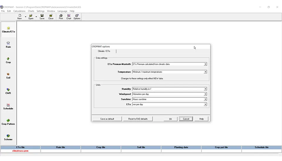
The Climate/ET0 window has its own Option window. In this window we can change data settings and units. In the Data Setting section, we can select that ET0 Penman-Monteith calculated from climate data or temperature data. Also about the section Temperature, we can select Minimum/Maximum Temperatures or Average Temperatures. In the Units section, there are humidity, wind speed, sunshine, and ET0. In the Humidity section, we can consider the relative humidity in percentage or vapor pressure in KPa. For the Wind Speed Section, we can select kilometers per day (more common) or meters per second. We have three options in the sunshine section. The first one is based on hours of sunshine. The second option is a percentage of daylength, and the last is a fraction of daylength. The next part in the Units section is the evaporation and transpiration potential of the reference plant (ET0). The ET0 can be in millimeters per day or millimeters per period. If you want, it is possible to save these changes as defaults. Additionally, in the CROPWAT options, there is an option called reset to FAO defaults if you want to go back to the default settings of FAO in this software. You can see these items in figure 9.
Fig. 9. CROPWAT Options (Climate/ET0)
1.3.1.2. Climate/ET0 Charts
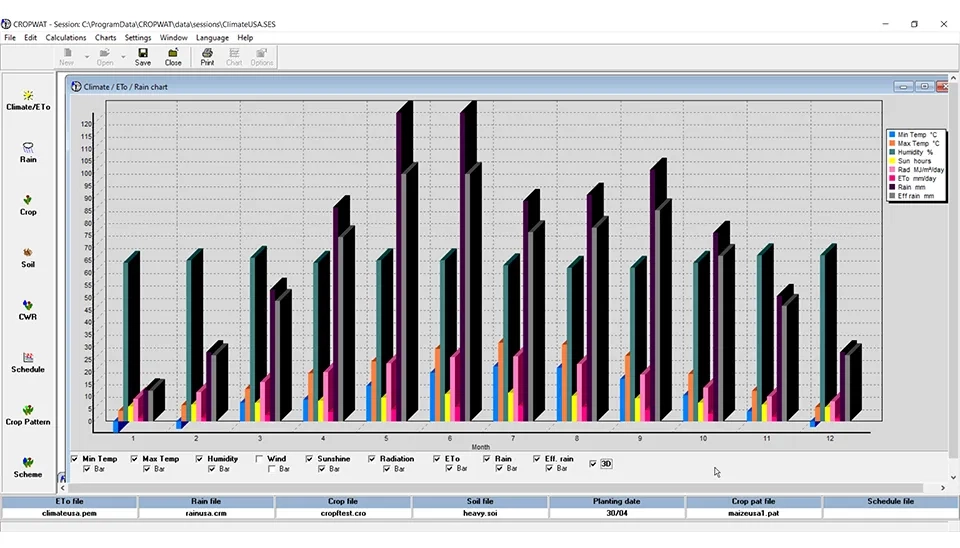
In the Climate/ET0 section, it is possible that you see the results as graphs. The graphs are based on monthly data. For displaying these graphs, you can enable options. The options are minimum temperature, maximum temperature, humidity, windspeed, sunshine, radiation, and ET0 (calculated by CROPWAT in Climate/ET0 Section), as well as rain and effective rainfall (calculated by CROPWAT in the Rain section). We enable all options for display graphs except the wind speed graph because of its high difference between its values and other parameters . You can see that in figure 10.
Fig. 10. Monthly Climate, ET0, and Rain Graph
According to figure 10, the highest average of the minimum and maximum temperatures, sunshine in hours, ET0 and radiation are in July. The highest percentage of humidity is related to November and December. The highest amount of rain is in the months of May and June. You can see the graphs related to rain and effective rain in the next section, which shows rain data separately. And now we represent the monthly wind speed graph in figure 11.
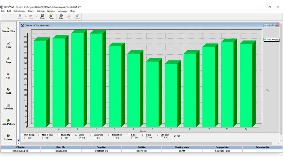
Fig. 11. Monthly Wind Speed in CROPWAT application
Figure 11 shows that wind speed is highest in March and lowest in August, reflecting seasonal variations, assuming other factors remain constant. The higher wind speeds in March can increase evapotranspiration, leading to higher water loss, while the lower wind speeds in August reduce this effect.
1.2.2. Rain
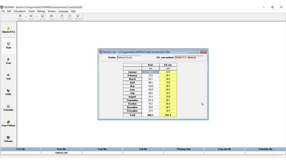
The second section is related to Rain. In this step we enter the station name and rainfall calculation method, and we also enter monthly rainfall as shown in Figure 12. As mentioned before, we can use the CLIMWAT software to enter the data related to the rain. In this project, we use the data from a weather website (see section 1.1)
Fig. 12. Monthly Rainfall Input in the Cropwat Software
The method for calculating rainfall in CROPWAT can be adjusted through the "Options" menu, allowing users to select the most suitable approach for their specific conditions. Once the desired method is chosen, the software automatically computes the effective rainfall, as displayed in the yellow column. Further details about adjusting and selecting the effective rain calculation method are explained in the following section, ensuring users can tailor the process to align with their needs and achieve accurate results.
1.2.2.1. CROPWAT Rain Options
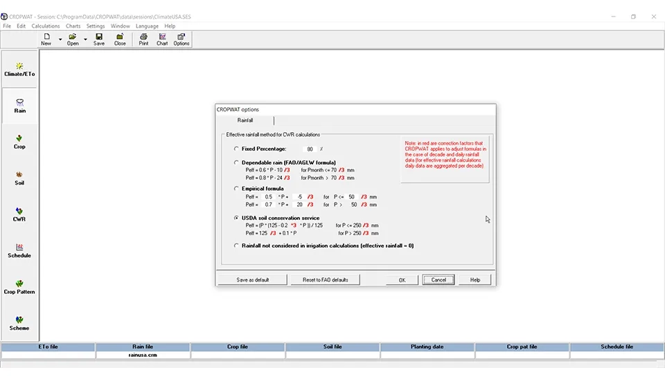
In this section, we can select one of these four methods for calculating effective rainfall. The first method is fixed percentage, which is 80 percent by default, but it can be changed manually. A fixed percentage equals 80%, which means that 80% of rainfall is effective. The second method is the dependent rain formula. And the third method is the empirical formula. The fourth method is FAO’s recommended method, USDA soil conservation service. The last method has stated rainfall is not considered in irrigation calculations (effective rainfall = 0). You can see the CROPWAT rain options in Figure 13.
Fig. 13. CROPWAT Rainfall Options
َAs before, there are two options: Save as default and Reset to FAO defaults.
1.2.2.1 Monthly Rain and Effective Rainfall Charts
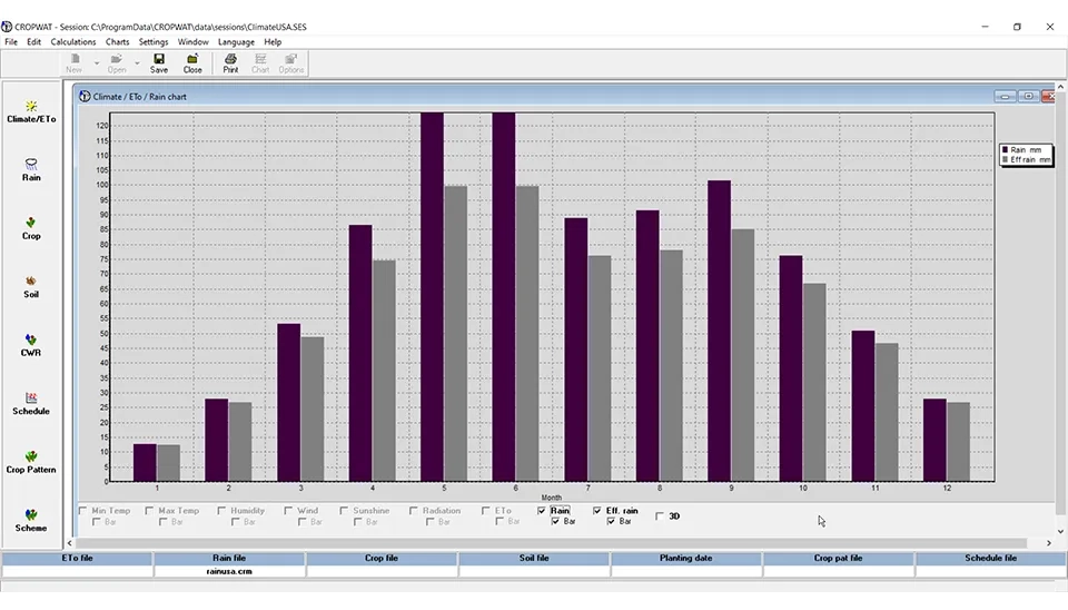
As mentioned before, at this step, you can see just the rain and effective rain in one graph, as shown in figure 14. This graph shows the monthly distribution of total rainfall (rain) and effective rainfall (Eff. rain) throughout the year. The dark purple bars represent total rainfall (in mm), while the gray bars represent effective rainfall, which is the portion of rainfall that is actually usable by crops after accounting for losses like runoff and deep percolation.
Fig. 14. Monthly Rainfall and Effective Rain graphs in CROPWAT Application
Rainfall is highest in late spring and early summer, with a peak in May and June. During these months, the effective rainfall also reaches its maximum, but it is consistently lower than the total rainfall, indicating that not all rainfall contributes directly to crop water availability. In the summer months (July to September), both total and effective rainfall decrease, which could suggest a potential need for additional irrigation to supplement the reduced effective rainfall.
1.2.3. Crop
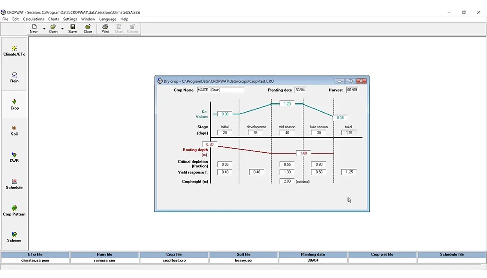
After entering the data related to Climate/ET0 and rain, whether using the CLIMWAT software or using the other data that you have, the next step is to enter the plant type and plant coefficients, as shown in figure 15. This part is including:
Fig. 15. Implementing Dry Crop Data in CROPWAT software
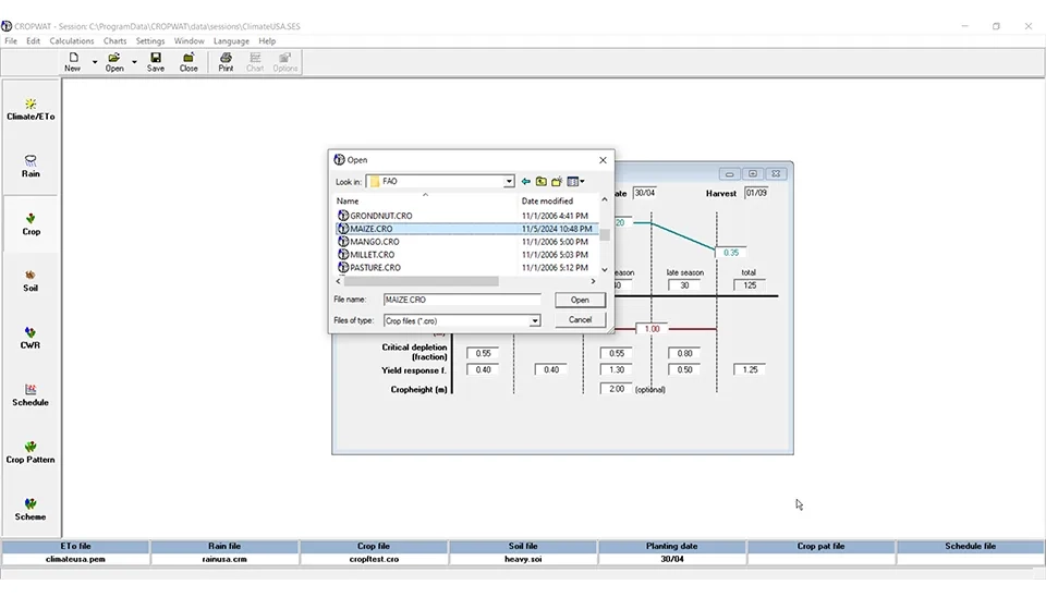
Crop name: We can select a crop from the FAO defaults (for example, maize (grain)), but how can we do this? While the crop window is opened, we select Open from the File menu, as shown in the following figure, to access different types of plants and their coefficients in the FAO file. By selecting a type of plant, other required coefficients of this section are determined automatically, but we can enter data manually if it is available. In that case, the data will be obtained with the help of equations and tables in FAO Irrigation and Drainage Paper 56. In the following, we explain other parts of this Crop window (Figure 16).
Fig. 16. Selecting FAO Crops Names and Crop Coefficients in Crowat
Planning date: we should enter the day and month of planning manually.
Harvest: Harvest is calculated by the CROPWAT software itself.
Kc Values: It is the plant coefficient, and it is calculated by the CROPWAT software automatically in this project.
Stages (days): It is related to the stages of plant growth in days and divided into four stages. The first is the initial stage, the second is the development stage, the third is the middle season, and the last stage is the late season.
Rooting depth (m): It is the plant root depth.
Critical depletion (fraction): According to FAO, the critical depletion represents the critical soil moisture level where first drought stress occurs affecting crop evapotranspiration and crop production.
Yield response f.: The yield response factor, or (Ky) are crop specific. Ky values vary over the growing season according to growth stages.
Cropheight (m): Cropheight is one of the crop factors.
It is emphasized that you can use the CROPWAT software defaults (for steps 4 to 9) instead of using FAO Irrigation and Drainage Paper 56.
1.2.4. Soil
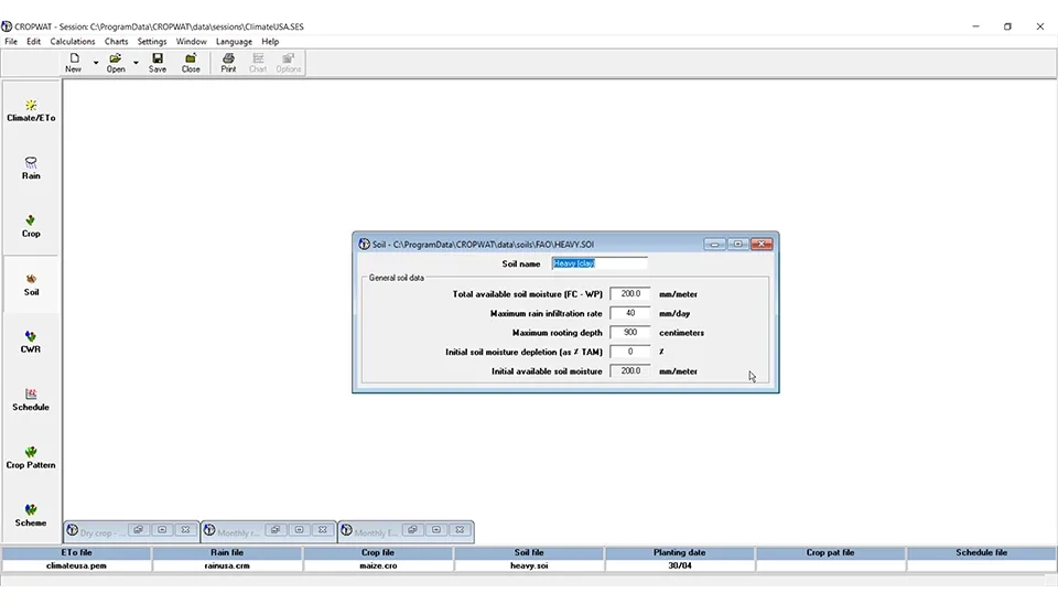
In the next section, we selectthe soil type, which is determined according to the region. Just like previous steps, we can use the CROPWAT software defaults and specify the desired soil type. In this project, we considered the heavy clay as the type of soil. To select this type of soil, as before, while the soil window has been opened, we go to File from the menu bar and select Open. Now we access FAO defaults. You can see data related to this section in figure 17 (Johnson County Kansas).
Fig. 17. Soil Data input in The CROPWAT
In this window we have these items:
Soil Name: for Overland Park, the soil name is Heavy (Clay);
Total available soil moisture (FC-WP): 200.0 mm/meter
Maximum rain infiltration rate: 40 mm/day
Maximum rooting depth: 900 cm
Initial soil moisture depletion: 0%
Initial available soil moisture: 200.0 mm/meter
Steps 2 to 6 are filled automatically after selecting the soil name from the FAO file in the CROPWAT software, just as was done in this project. But it can be calculated with the help of FAO Irrigation and Drainage Paper 56, manually.
1.3. Outputs
In this section, we explain the outputs of the CROPWAT software, including CRW, Schedule, Crop Pattern, and Scheme. So by reviewing the results, we can find out the crop water requirements and obtain an irrigation schedule and scheme supply.
1.3.1. Crop Water Requirement (CRW)
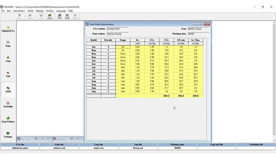
This section is Crop Water Requirements and is calculated according to all the previously saved data by the CROPWAT software itself. You can see these results as shown in figure 18.
Fig. 18. Monthly Crop Water Requirement Results table
In figure 18, each cultivation month is divided into three decades. The plant growth stages in each decade of the month are specified. In the next column, plant coefficients are displayed. The crop evapotranspiration, or ETc, is also displayed in two different units: millimeters per day and millimeters per decade. The effective rain in millimeters per decade is shown. The last part is related to irrigation requirements in millimeters per decade. According to this table, the highest irrigation requirement is in the third decade of July. The crop evapotranspiration (ETc) in millimeters per decade computes 609.3. The effective rain is 359.4 millimeters per decade. Irrigation requirements were obtained at 299.8 millimeters per decade throughout the planting period.
13.1.1. Crop Water Requirement Chart
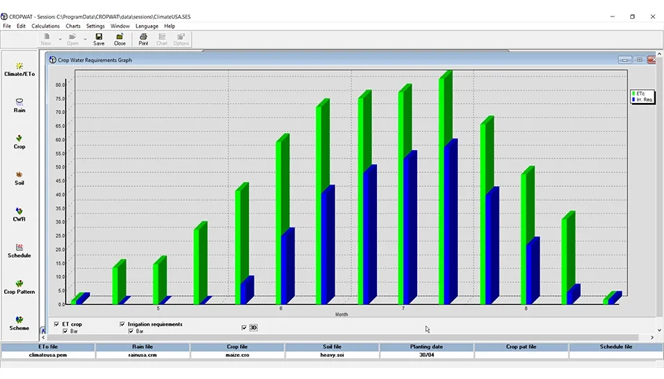
In this step, we can also have the monthly crop water requirement and the crop evapotranspiration (ETc) in graphs. You can see the ET crop and Irrigation Requirements graph for Maize (grain) plant in figure 19.
Fig. 19. ETc and Monthly Irrigation Requirements graph
This graph represents decade-based data, where the horizontal axis is divided into decades within each month, providing a finer temporal resolution for analyzing crop water requirements. Each month is split into three decades, representing the first, second, and third 10-day periods. The green bars indicate crop evapotranspiration (ETc), which measures the water lost through both transpiration from the crop and evaporation from the soil. When effective rainfall is insufficient, additional water is required to meet crop demands, as indicated by the blue bars that represent irrigation requirements.
The data reveals that both ETc and irrigation requirements peak during the third decade of July, a critical growth stage for the crop when its water demand is at its highest. This suggests that the crop requires significant supplemental irrigation during this period to prevent water stress and ensure optimal growth and yield. The decade-based structure of the graph allows for more detailed tracking of water needs, enabling better alignment of irrigation schedules with the dynamic water requirements of the crop throughout the growing season. This precise representation underscores the importance of monitoring and managing water resources effectively to sustain agricultural productivity, particularly during periods of peak demand.
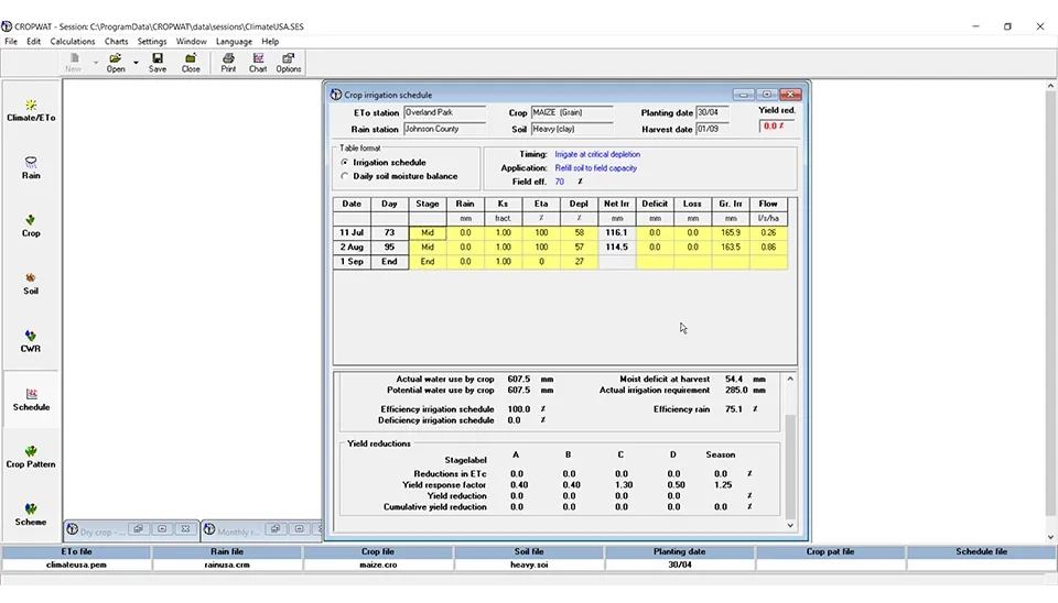
1.3.2. Schedule
The next output is related to the schedule. In this section, we can see the crop irrigation schedule as shown infigure 20. At the top of the crop irrigation schedule, we can see the ET0 station (Overland Park), the selected plant name (Maize (grain)), the planning date (30/04), the yield reduction (0.0%), the rain station (Johnson County), the soil (heavy clay), and the harvest date (01/09). Through a number of earlier steps, we inputted all of this data into the CROPWAT software.
Fig. 20. Crop Irrigation Schedule
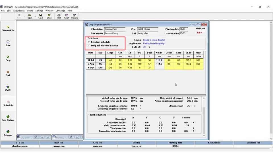
In figure 21, we have specified the table format. In the section of Table format, we can select one of two output options. Either irrigation schedule or daily soil moisture balance. First we show the irrigation schedule case and introduce other sections.
Fig. 21. Irrigation scheduling (Table format -Schedule tab)
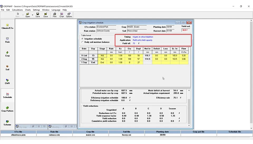
In the next section of the schedule window, shown in figure 22, we find out when and how much water to apply to a field. The timing is in response to when to apply in this project and it is considered to irrigate at critical depletion when the Reality Available Water (RAW) is totally depleted.
Fig. 22. Timing, Application, and Field Efficiency (Percentage) in the Cropwat Software
The application is in response to how much to apply, Refill soil to field capacity if you intend to refill soil to field capacity (FC). Field efficiency is 70 percent, although you can change all of these parts in the CROPWAT Options window as in the following section.
According to figure 22, on the 11th of July or 73 days after cultivation, the net irrigation is 116.1 mm and on the second of August or 95 days after cultivation, the net irrigation is 114.5 mm.
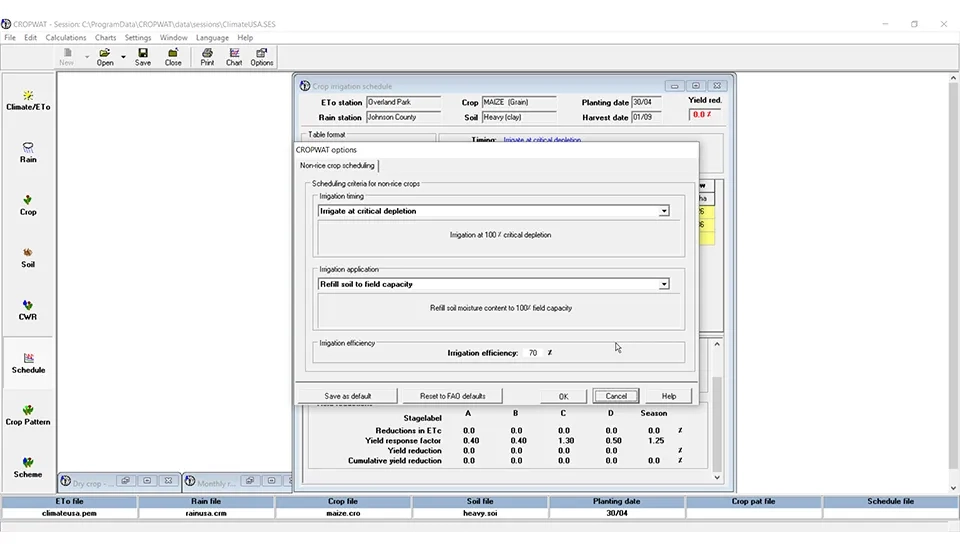
1.3.2.1. Options
In this section (Figure 23), we can change the depletion timing. Its options are irrigation at user defined intervals (days), Irrigation at critical depletion (100% of RAW), Irrigation below or above critical depletion (percent of RAW), Irrigation at fixed interval per stage (10 days in each stages), Irrigate at fixed depletion (40 mm), Irrigation at given ET crop reduction (10% in each stage), Irrigation at given yield reduction (10%), No irrigation (rainfed). In the next part, we can change the irrigation application so that it can be User defined application depth(mm), Refill soil to field capacity (100% FC), Refill soil below/ above soil capacity (percent of depth FC), Fixed application depth (40 mm) and the next option is depending on irrigation efficiency which you consider. Irrigation efficiency is based on the type of irrigation system.
Fig. 23. CROPWAT Non-Rice Crop Scheduling Options
You can have more details in FAO Irrigation and drainage Paper No.56. The schedule window indicates: Date, Day, Stage, Rain (mm), Water stress coefficient (KS), Crop evapotranspiration under non-standard conditions (ETc adj), Root zone depletion, Net irrigation deficit (amount of water in millimeter below field capacity), Irrigation losses, Gross irrigation and Flow (l/s/h). The flow is the continuous water discharge needed to satisfy crop irrigation requirements over the irrigation interval period. It is expressed in liters per second per hectare and calculated by converting the gross irrigation application depth into a permanent supply.
Fig. 24. Totals and Yield Reductions (Schedule tab)
In the bottom of the window is represented the Totals. This section contains Total gross irrigation. The total grass irrigation is the sum of the column related to Grass irrigation. The total Net irrigation is 230.6 that you can see the values of in the Net irrigation column. The total irrigation losses is 0.0 mm because there were not any Losses. Now we can activate the other format in the Total format section that we mentioned before. So we activate the Daily soil moisture balance to know how the CROPWAT software computes the values of Total irrigation. Please look at the figure 25.
According to the above figures the values of Rain come from the rain column. Total rain loss is the difference between two Total rainfall and Effective rainfall in mm. Actual water use by crop is 607.5 mm. Potential water use by crop is 607.5 mm, too. Moist deficit at harvest is 54.4 mm. Actual irrigation requirement computed 285.0 mm. Efficiency irrigation schedule is 100%. So the deficiency irrigation schedule is 0.0%. Efficiency rain is: Total rainfall/ Efficiency rainfall * 100 So in this project the Efficiency rain has been 75.1%, also in the bottom box (figure 25), in the Crop Irrigation Schedule you can see other information like Yield reductions. The yield reductions are Stageslable, Reductions in ETc, Yield response factor, Yield reduction and Cumulative yield reduction.
You can have more details about this section, if you use the Help of the CROPWAT software according to the following path:
Notice that the Rice scheduling is special and is different from all of the things that are mentioned in this project.
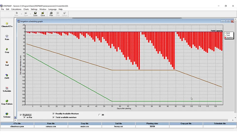
1.3.2.2. Irrigation Scheduling Graph
In this section, we also can have graphs called soil water retention (in mm) - Days after planting. In these graphs we can see Depletion, also, the red line represents Readily Available Moisture (TAM) and the green line represents Total available moisture (RAM).
Fig. 26. Irrigation Scheduling Graph in the CROPWAT Software
The irrigation scheduling graph in Figure 26 illustrates a clear trend in the TAM and RAM throughout the cultivation period. Initially, there is a noticeable decrease in TAM up to the 55th day after planting, reflecting the crop’s increasing water demand during this critical growth phase. Beyond this point, TAM stabilizes, maintaining a steady trend for the remainder of the cultivation period. Similarly, RAM exhibits a decreasing trend until the 55th day after planting. Following this, it remains relatively stable for approximately 40 days before resuming a gradual decline towards the end of the growing season. This pattern highlights the dynamic changes in soil moisture levels in response to crop water uptake and emphasizes the importance of well-timed irrigation to sustain optimal growth and prevent water stress during critical developmental stages.
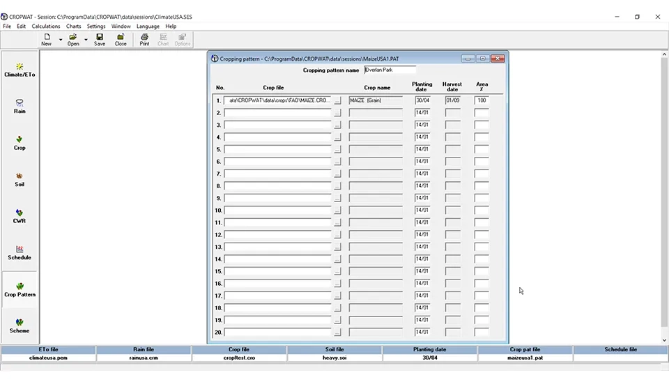
1.3.3. Crop Pattern
In this section, we can manage the planting of several types of plants together. In this project, we considered that 100% of the farm is cultivated. You can see these data in the following figure.
Fig. 27. Cropping Pattern in the CROPWAT application
According to figure 27, we enter a name for the cropping pattern. For the Crop file, we should select the crop file by clicking on the three-dot icon to open the FAO file. Other parts, including Crop name, Planting date and Harvest date are loaded automatically by the CROPWAT software. Now it just needs you to enter a percentage of the area that the selected crop is planted in that area. If we have other crops, we will do the same again.
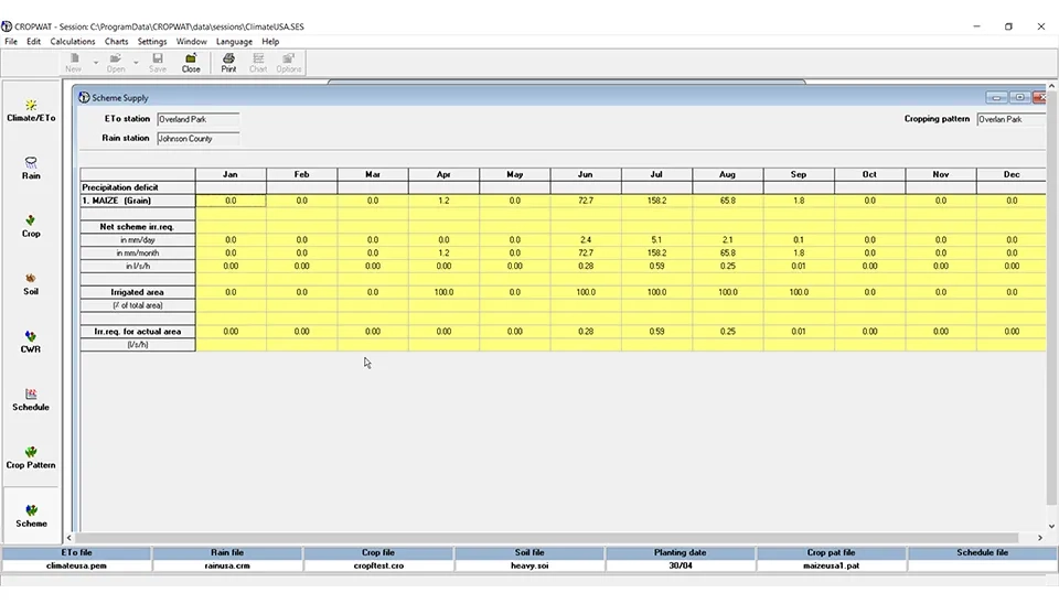
1.3.4. Scheme
The last section is Scheme. The scheme provides information for each month’s water supply. You can see the information on the water supply for this project in figure 28. In this section, we have the difference of months of year and precipitation deficit in these months. These values come from consideration by the crop water requirements window. Actually, those are the monthly summations of irrigation requirements in mm/dec (millimeters per decade). You can check it yourself to find out the numbers correctly and make sure!
Fig. 28. Scheme Supply in the CROPWAT System
After that, we have Net Scheme irrigation requirements in three different units (mm/day, mm/month, and liter per second per hectare). For example, in the net scheme irrigation requirements in mm/month, simply multiply the numbers for precipitation deficit for each month by the planting area that you specified in the step crop pattern window previously.
The next is irrigated area, which means the percent of total area. We are just talking about the crop pattern, and we specify that for the maize (grain), we have considered the entire area as the cultivation area.
The last output in this window is the presented irrigation requirement for the actual area in (l/s/h). To find out where these numbers come from, simply divide the numbers for net scheme irrigation requirements in l/s/h (pay attention to the unit) and divide the numbers: Irrigation area (for this project, the whole of the area is cultivated; the number of irrigation areas is 100% or 1).
Notice that if you do all of the steps correctly, in the status bar at the bottom of the main window in this section, you can see the status of each step.
2. Conclusion
In this article, considering the importance of saving water resources, we have explained the different sections of the CROPWAT software for estimating the water requirement of corn plants in Overland Park. The software consists of four input tabs, and we have explained step by step how to work with the software in these different sections.
It was also mentioned that CROPWAT has four output tabs. Based on the output, for corn plants in the Crop Water Requirement (CWR), considering an effective rainfall of 609.3 mm/dec and evaporation of 359.4 mm/dec, the irrigation required during the cultivation period was obtained as 299.8 mm/dec.
It was also found that in schedule output, net irrigation 73 days after planting was 116.1 mm and 95 days after planting, i.e., on August 2, was 114.5 mm. And we explained that it is possible to manage different types of cultivation in an area using the crop pattern tab. And finally, a monthly scheme supply is provided as the last output.


-678e80e72f45fbd642a0fe13)
-678e81352f45fbd642a0fe17)


Comments
No comments yet
Be the first to comment
Share your thoughts and start the conversation.