Remote Sensing Techniques for Evapotranspiration Analysis: A Review
It is estimated that the global average annual Evapotranspiration (ET) is approximately 505,000 cubic kilometers of water per year. This amount of water is ten times what is required to produce enough food and drinking water for everyone.
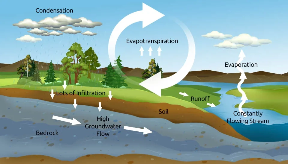
How much water does the world lose annually to evapotranspiration? It is estimated that the global average annual Evapotranspiration (ET) is approximately 505,000 cubic kilometers of water per year. This amount of water is ten times what is required to produce enough food and drinking water for everyone. On the other hand, evapotranspiration plays a crucial role in linking the global energy, water, and biogeochemical cycles, and it helps to understand how ecosystems respond to global environmental changes (Bhattarai and Wagle, 2021). Due to the impossibility of directly estimating evapotranspiration and it is collective of several terms such as evaporation and transpiration from vegetation and soil, remote sensing techniques are employed to assess these processes on a large scale (Liou et al., 2014). Remote sensing is widely acknowledged as the sole practical method for mapping regional and mesoscale patterns of evapotranspiration on the Earth’s surface in a globally consistent and economically feasible manner, and surface temperature helps to establish the direct link between surface radiances and the components of surface energy balance (McCabe and Wood, 2006). Figure 1 shows the cycle of evapotranspiration on the Earth.
Fig. 1. Role of Evapotranspiration in Earth’s Dynamic Processes
Table 1. Comparisons of a variety of commonly used satellite-based evapotranspiration assessment methods
Methods
Inputs
Main assumptions
Advantages
Disadvantages
Simplified Method
Rnd, Ts, Ta
1) The daily soil heat flux is negligible
2) Instantaneous H at midday can express the influence of partitioning daily available energy into turbulent fluxes
Simplicity
Site-specific
Residual Methods
Based
SEBI
Tpbl, hpbl, u, Ts, Rn, G
1) The dry limit has a zero surface ET
2) The wet limit evaporates potentially
Directly relating the effects of Ts and ra on LE
Ground-based measurements are needed
Based S-SEBI
Ts, as, Rn, G
1) EF varies linearly with Ts for a given surface albedo
2) Ts, max corresponds to the maximum LE
3) Ts, min corresponds to the maximum LE
No ground-based measurements are needed
Extreme temperatures have to be location-specific
Based SEBAL
u, Za, Ts, VI, Rn, G
1) Linear relationship between Ts and dT
2) ET of the driest pixel is 0
3) ETwet is set to the surface available energy
1) Minimum ground measurements
2) Automatic internal calibration
3) Accurate atmospheric corrections are not needed
1) Applied over flat surfaces
2) Uncertainty in the determination of anchor pixels
1. Evapotranspiration and The Earth System
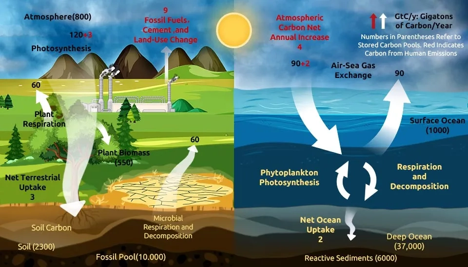
Around two-thirds of precipitation that falls on land surfaces is released back into the atmosphere through ET (Chen et al., 2020). ET is widely recognized as the most crucial process in the Earth system as it links the water cycle, carbon cycle, and surface energy budget (Fisher et al., 2017). Plants open their stomata during photosynthesis to absorb CO2, which facilitates the simpler release of water into the atmosphere at the cost of significant energy expenditure to turn liquid water into vapor (Fisher et al., 2017). Globally, on land surfaces, ET is the second-largest process in the terrestrial water cycle, returning approximately two-thirds of water from precipitation back to the atmosphere (Chen et al., 2023). Therefore, any changes in evapotranspiration have significant implications for water storage, potential runoff, the carbon balance of a region (whether it acts as a source or sink of carbon), and the regulation of the surface energy budget. These changes also play a role in mitigating or exacerbating heat waves (Wolf et al., 2016).
when the temperature rises due to increasing greenhouse gases, the saturated pressure of the atmosphere increases, leading to a high vapor pressure deficit between wet surfaces and the air above them (Yuan et al., 2019). Changes in evapotranspiration play a crucial role in influencing the distribution of water availability and carbon uptake (Zhao et al., 2022). Therefore, models of ET are needed to understand how changes in water availability, land cover, human management, and climate impact the energy, water, and carbon cycles within the Earth system (Sorooshian et al., 2011). Satellite-based evapotranspiration assessment can be employed to evaluate the impacts on local and regional climate (Lo and Famiglietti., 2013; Sorooshian et al., 2011).
Figure 2. A schematic representation of the global water and carbon cycles, highlighting the crucial role of evapotranspiration in linking these essential Earth systems.
2. Satellite-Based Evapotranspiration Assessment
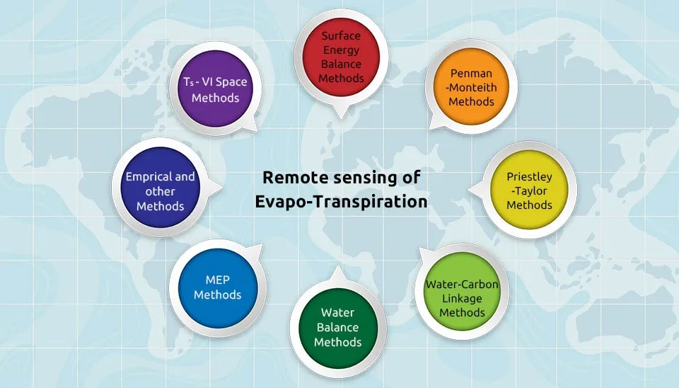
How has satellite technology facilitated the monitoring of evapotranspiration? Satellites offer global measurements of vegetation properties, land surface temperature, soil moisture, and changes in total water storage. These satellites provide spatial resolutions and frequencies crucial for accurate evapotranspiration mapping (Corbari et al., 2020). Algorithms of remote sensing for evapotranspiration estimation use satellite observations related to land surface variables to calculate the spatial distribution of evapotranspiration (Mu et al., 2011). Various methods have been developed to estimate reference and plant evapotranspiration using satellite images. This method has its complexity generally. Figure 3 shows different methods of measuring evapotranspiration. This paper examines some of the methods for estimating evapotranspiration using satellite data.
Fig. 3. Remote sensing application for evapotranspiration estimation
2.2. Simplified Empirical Regression Methods
The simplified empirical method utilizes the principles of energy balance to determine evapotranspiration. The components of land surface energy balance involve interactions such as radiative exchange with the atmosphere, the transfer of heat through the ground, and the exchange of latent and sensible heat fluxes with the lower atmosphere, characterized by turbulence (Haghighi et al.,2018). Therefore, evapotranspiration with an energy balance model is,
RN, G, H, are the flux densities of net radiation, soil heat, and sensible heat flux. Total daily evapotranspiration (LE) is estimated using surface temperature measurements obtained remotely at a specific time of day. This estimation is done through the application of a statistically established formula. Based on studies, the following equation is proposed for this purpose (Muran and Jackson., 1991).
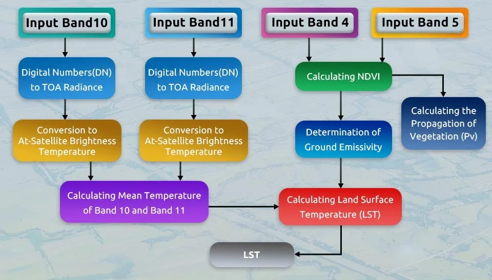
This equation is obtained from the difference between instantaneous surface temperature (Ts) and air temperature (Ta). Moreover, LEd, Rnd, B and n represents evapotranspiration, net radiance, site-specific regression coefficients depending on surface roughness, wind speed, atmospheric stability, etc. Surface temperature, atmospheric temperature, and net radiation values are obtained using satellite data. Figure 4 shows how to calculate the surface temperature using the combination of 4, 5, 10, and 11 of the Landsat 8 satellite. NDVI is the vegetation index.
Figure 4. Estimating Land Surface Temperature for Satellite-Based Evapotranspiration Assessment
2.2. Residual Methods of Surface Energy Balance
The residual methods of surface energy balance are extensively used for mapping ET at different temporal and spatial scales. It is divided into two categories: 1) single-source and 2) dual-source models (Bhattarai et al., 2016).
2.2.1. Single-Source Models
The essential feature of integrated single-source methods is the assumption of the surface, which is based on the comparison between wet and dry methods. The relationship of the single-source model is energy balance.
LE = RN - G - H
In the above equation, RN, G, and H are estimated by integrating surface radiometric temperature and shortwave albedo measurements obtained from visible, near-infrared, and thermal infrared wavebands through remote sensing techniques. In the following section, we show how to calculate each one (Gowda et al., 2008).
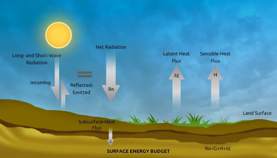
2.2.1.1. Net Radiation Equation (RN)
Net radiation is a crucial parameter used in calculating reference evapotranspiration and serves as a driving force in numerous physical and biological phenomena. To assess the daily net radiation across a plant canopy, the approach involves utilizing canopy temperature, albedo, and solar radiation (Samani et al., 2007).
The surface shortwave albedo ∝s is typically derived by the combination of narrow-band spectral reflectance values from remote sensing bands. Rs is determined by various factors such as the solar constant, solar inclination angle, geographical location, time of year, atmospheric transmissivity, and ground elevation (Allen et al., 2007). The elevation of surface emissivity εs involves determining a weighted average between bare soil and vegetation (Li and Lyons, 1999) or as a function of the Normalized Difference Vegetation Index (NDVI) (Bastiaanssen et al., 1998), εa is atmospheric emissivity and estimated as a function of vapor pressure (Brutsaert et al., 1975).
Fig. 5. Surface Energy Budget illustrating the key components involved in evapotranspiration Net Radiation (Rn), Soil Heat Flux (G), Sensible Heat Flux (H), and Latent Heat Flux (LE).
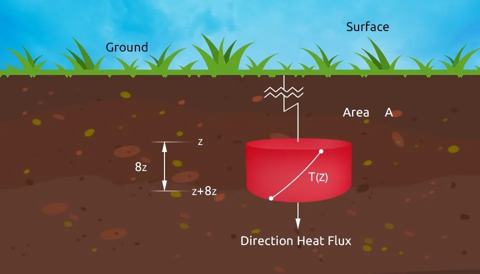
2.2.1.2. Soil Heat Flux (G)
Directly mapping the G, or soil heat flux component through satellite observation is not feasible. However, the fraction G/Rn can be reasonably estimated around nouns using empirical relationships derived from satellite image data that capture soil and vegetation characteristics. These characteristics include the leaf area index (LAI), normalized difference vegetation (NDVI), albedo, and land-surface temperature (LST). Consequently, several models have been proposed to estimate G based on the G/Rn ratio, incorporating soil and vegetation characteristics (Danelichen et al., 2014).
Therefore, the assumption that the daily value of G is equal to 0 and can be negligible in the daily energy balance is generally considered a reasonable approximation (Price, 1982).
Fig. 6. Soil heat flux direction used for satellite-based evapotranspiration assessment
2.2.1.3. Sensible Heat Flux (H)
H, or sensible heat flux, is the heat transfer between the ground and atmosphere. Solely relying on remote sensing approaches for estimating sensible heat flux is insufficient since many models integrate micrometeorological and RS concepts. While RS models primarily use land surface temperature as the primary boundary condition, they do not consider uncertainties caused by canopy cover and atmospheric turbulence. Parameters such as surface roughness and wind velocity become crucial, particularly under non-neutral atmospheric conditions. Consequently, estimating H requires a hybrid approach that incorporates both RS and micrometeorological concepts (Mohan et al., 2020).
Aerodynamic resistance ra is affected by the combined factors of surface roughness (vegetation height, vegetation structure), wind speed, and atmospheric stability (Courault et al., 2005).
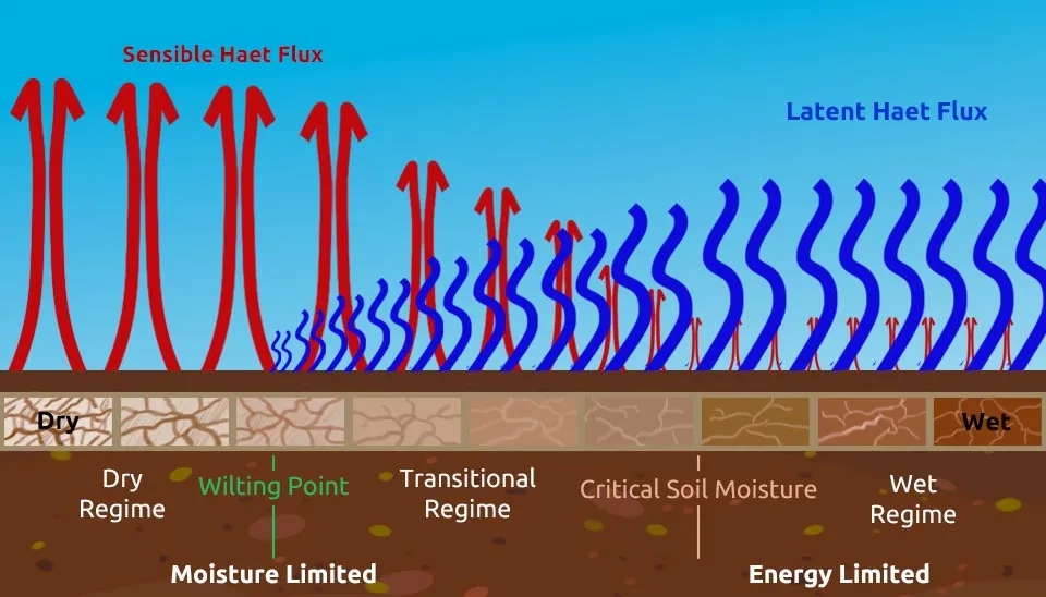
The primary difference among different approaches in single-source surface energy balance models is the estimation of sensible heat flux. Some methods utilize spatial contextual information, such as identifying characteristics of dry and wet pixels within regions of interest and land surface properties (Li et al., 2009). Below is an overview of several notable single-source energy balance models.
Fig. 7. Enhancing evapotranspiration estimation through satellite data innovations by utilizing sensible and latent heat flux of dry and wet earth.
1) Surface Energy Balance Index (SEBI)
The Surface Energy Balance Index (SEBI) was devised to estimate evapotranspiration from the evaporative fraction by considering the differences between dry and wet regions. In this method, relative evaporation is determined by scaling an observed surface temperature within a maximum range of surface temperature. This range is indicated by the extremes in the surface energy balance, which provide theoretical lower and upper limits on the difference between surface and air temperatures. Under specific conditions, when water availability in the soil is limited and certain boundary layer characteristics are met, evaporation is assumed to be zero. In such cases, the sensible heat flux density reaches its maximum value. Ts,max is inverted from the bulk transfer equation (Liou and Kumar., 2014),
the minimum surface temperature can be determined by considering the wet limit, where the surface is assumed to have the potential for evaporation. The potential evapotranspiration can be calculated using the Penman-Monteith with zero internal resistance. The surface temperature (T) is expressed as follows:
The relative evaporation fraction can then be calculated using interpolating the observed surface temperature within the maximum and minimum surface temperature in the following form:
The second part of the right-hand side of the above equation is the so-called SEBI, which varies between 0 (actual = potential ET) and 1 (no ET).
2) Simplified SEBI (S-SEBI)
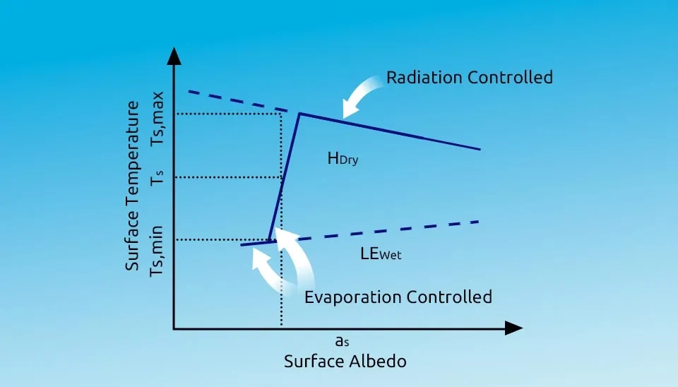
The S-SEBI model primarily establishes a maximum temperature for dry conditions based on reflectance and a minimum temperature for wet conditions also determined by reflectance. Afterward, the model allocates sensible and latent heat fluxes based on actual surface temperature (Roerink and Menenti, 2000).
This model is theoretically explained in the context of a wide range of surface characteristics transitioning from dry or dark soil to wet or bright pixels. The explanation can be outlined 1) In areas with low reflectance (albedo), the surface temperature remains relatively stable due to sufficient water available under these conditions, such as over open water or irrigated lands; 2) As reflectance (albedo) increases, the surface temperature rises to a certain point. This increase in temperature is attributed to decreased evapotranspiration caused by reduced water availability This condition is referred to as “evaporation controlled”. 3) after the inflection point, the surface temperature decreases as surface reflectance continues to increase. This phenomenon is termed "radiation controlled” (Zhao-Liang Li et al., 2009 ).
Fig. 8. Theoretical schematic relationship between surface temperature and albedo in the S-SEBI model.
To estimate evapotranspiration using this method, the initial step involves calculating the fraction of evapotranspiration between temperature corresponding to dry (TH) and wet (TLE) conditions.
Where (Λ) is an evaporative fraction, and Ts is the land surface temperature (Sobrino et al., 2021). Once Λ is obtained, LET with knowledge of net radiation and soil heat flux can be obtained according to
3) Surface Energy Balance Algorithm for Land (SEBAL)
SEBAL, is a technique developed by Bastiaanssen to estimate evapotranspiration using minimal reliance on ground-based measurements. It has been tested in various climates across more than 30 countries worldwide, in both field and catchment scales (Bastiaanssen et al., 1998). Across different soil wetness and plant community conditions, the typical accuracy of SEBAL at the field scale is 85% for a single day, which further improves to 95% throughout a season (Bastiaanssen et al., 2005).
The main advantage of the SEBAL model is that overcomes the challenges associated with accurately estimating the true values of aerodynamic temperature (Taero) and air temperature at reference height (Ta). It achieves this by assuming a linear correlation between the temperature difference (dT) of Taero and Ta with the land surface temperature Ts.
Where a and b are empirical coefficients derived from two anchor points (dry and wet points).
At the dry pixel, latent heat flux is assumed to be zero, and the surface-air temperature difference at this pixel is obtained by inverting the single-source bulk aerodynamic transfer equation.
Where ρ and Cp are air density and specific heat capacity of air, respectively; ra is aerodynamic resistance to heat transport, which is determined by iteration of air stability corrections (Bastiaanssen., 2000).
In the initial estimation of H, a neutral atmospheric condition is assumed, and the aerodynamic resistance to heat transfer is calculated using the following method:
Where z2 and z1 are height above the zero plane displacement of the vegetation where the endpoints of dT are defined; k is constant of von Karman; u is friction velocity calculating using the following equation:
Where u200 is wind speed at blending height, which is chosen to be 200 m in SEBAL. zom is momentum roughness length.
During subsequent iterations, the monin-Obukhow length (L) is calculated as a primary step to assess the atmospheric stability conditions.
Where g is gravitational acceleration.
Then, the corrected value for u and ra each iteration is calculated from the following equation:
Where ψm(200) is the stability correction momentum transport at 200m height. ψh(z2) and ψh(z1) are stability corrections for heat transport at heights z2 and z1. ψm and ψh are functions of Monin-Obukhov length (Yuting Yang et al., 2012).
2.2.2. Dual-Source Model
Although single-source energy models can offer dependable estimations of turbulent heat fluxes, they often necessitate field calibration and may have limited applicability across various surface conditions. In contrast, the dual-source model does not require pre-calibration and can be applied without additional ground-based information, unlike single-source models. However, in dual-source energy balance models, assumptions and solutions typically involve understanding the variations in surface energy balance within the canopy and considering the impact of clumped vegetation.
These factors influence the wind speed profile, radiation penetration, and the partitioning of radiative surface temperature between soil and vegetation (Andreson et al., 1997).
3. Conclusion
Remote sensing, with its incredible ability to capture a holistic view, has many advantages for evaluating evapotranspiration. Its prowess lies in its ability to offer a comprehensive understanding of the intricate processes governing water movement in ecosystems.
As mentioned, remote sensing has many advantages for evaluating evapotranspiration. On the other hand, different methods of estimating evapotranspiration using satellite data can show their application well in different conditions. In diverse environmental settings, satellite-based approaches prove their versatility, effectively adapting to the unique characteristics of each region.
However, remote sensing, like all other methods, has its disadvantages, such as problems related to remotely sensed data and the uncertainty of Remote sensing ET Models. Challenges arise in the form of data-related issues, introducing a layer of complexity to the precision of remote sensing outcomes. Additionally, uncertainties in the models used for ET assessment through remote sensing further emphasize the need for ongoing refinement and improvement in this dynamic field.
The evolving realm of remote sensing continues to be a beacon of promise for understanding evapotranspiration dynamics. The ongoing pursuit of overcoming challenges and refining methodologies ensures that remote sensing remains a powerful tool for unraveling the mysteries of water exchange in our intricate ecosystems.
Remote Sensing Techniques for Evapotranspiration Analysis: A Review | Waterlyst


Comments
No comments yet
Be the first to comment
Share your thoughts and start the conversation.