HBV-light for Hydrological Modeling: A Beginner's Guide
In today's world, hydrological modeling has become crucial, due to climate change the intensity and frequency of extreme events, such as floods has shifted. Therefore , it is necessary to study the behaviour of such events and one powerful tool for that goal is hydrological modeling.
In today's world, hydrological modeling has become crucial, due to climate change the intensity and frequency of extreme events, such as floods has shifted. Therefore , it is necessary to study the behaviour of such events and one powerful tool for that goal is hydrological modeling. A hydrologic model simulates a change of water storage with time within one or more components of the natural hydrologic cycle. These models provide insights into how changes in land use, vegetation, and climate affect the water cycle, thereby assisting policymakers and water resource managers in making informed decisions (Zarei et. al 2024). There are different types of hydrological models , including distributed and lumped models, based on how their parameters change spatially. Distributed models categorize the river basin to smaller parts to evaluate spatial variations in parameters, while lumped models see the whole river basin as one part, ignoring spatial differences. Working with lumped models is much easier than distributed models because they are less complicated and need minimum climatic data. One of the most popular lump models is HBV-light , which has frequently been used in hydrological studies with acceptable results and accuracy.
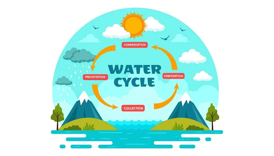
Fig. 1. The water cycle illustrates the continuous movement of water on, above, and below the surface of the Earth.
This article aims to provide a comprehensive guideline for using HBV-light software with a step-by-step guide from downloading the HBV-light software and observational data to the calibration process and getting the final results. This article is useful for researchers and students who want to use this model for hydrological modeling.
1. HBV-light
The Hydrologiska Byråns Vattenavdelning (HBV) model was originally developed byBergstrom and Forman in 1973 in the water balance section of the Swedish Meteorological and Hydrological Institute (SMHI) to facilitate hydropower operations in the 1970s. There are different types of HBV models; in this article we use HBV-light. The HBV model has three main hydrological processes: snow and snow cover, soil moisture and evaporation, and groundwater and response processes represented by two main reservoirs (
accumulation and melt in the snow princess part is vital for mountainous areas with snow affected and calculated as:
1:
2:
At the present time step Sn ,snow storage is calculated as the snow storage from the previous time step (Sn-1) plus the precipitation (P) minus the snowmelt (MS), which occurs when the air temperature exceeds a certain threshold. Precipitation is considered snow when the temperature is below the threshold, and the snowmelt (MS) is calculated based on the difference between the air temperature and the melting threshold (Jansen et al. 2021) . MSrate is the snow melt rate that is determined by the model. The snow storage Sn is updated at each time step, accounted for both the accumulation of snow and the loss due to melt.
The soil moisture process in HBV-light is divided into two reservoirs: the upper and lower soil moisture storage. Based on the soil moisture availability, the model calculates evapotranspiration (ET).
3:
Where the upper soil moisture storage (Su) is updated based on the precipitation that falls as rain (prain), the evapotranspiration from the upper soil layer (ETu), and the percolation (Qu) from the upper reservoir to the lower reservoir, which is groundwater. The change in Su is given by the difference between the incoming rain and the outgoing evapotranspiration and percolation, ensuring that the model captures the balance of water in the upper soil layer.
4:
The actual evapotranspiration from the upper soil layer (ETu) is calculated as a fraction of ET0, adjusted by a temperature-dependent function f(Tar). Additionally, the model uses the maximum storage capacity of the upper soil layer to scale the evapotranspiration.
5:
The change in Sl is determined by the percolation rate (Ql), which is a function of the moisture available in the lower soil layers, Therefore, linking the soil moisture storage with groundwater.
The groundwater in HBV-light represents the long-term water accumulation for base flow, which is considered as the total amount of quick response and low response as follows:
6:
Where Kquick is flow coefficient ofquick groundwater, and Sl is lower soil moisture.
7:
Similarly, Kslow is flow coefficient ofslow groundwater, and Sg.slow is lower soil moisture. Finally, runoff estimation is based on quick and slow groundwater flow and surface runoff. Transformation of soil moisture and groundwater storage into runoff, typically involving a nonlinear relationship.
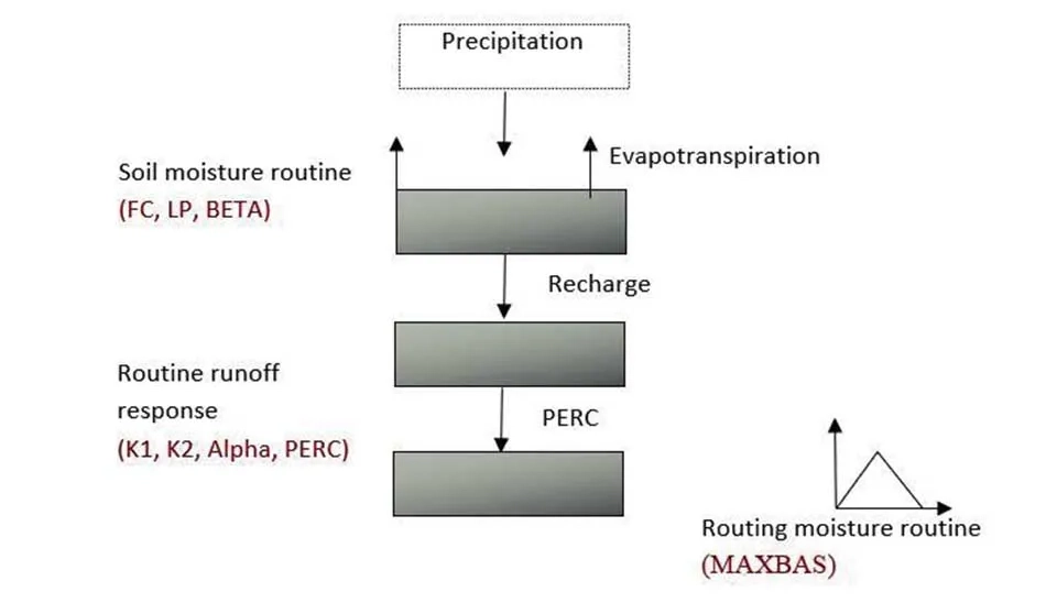
Fig. 2. Structure of the HBV-light model, illustrating the key components precipitation process, soil moisture process, and groundwater process.
2. Study area
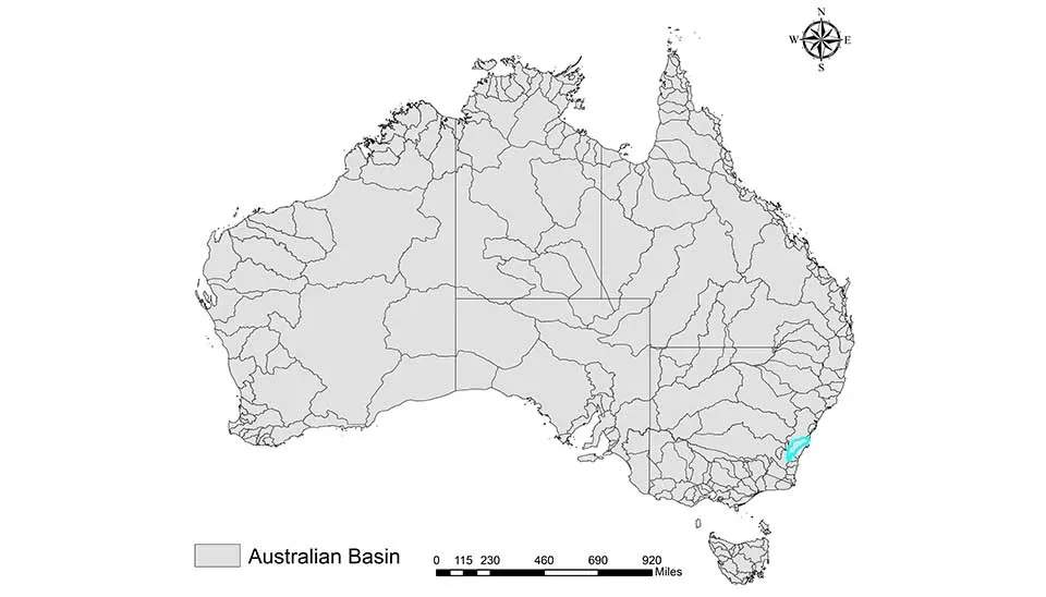
Various climate zones , including tropical regions in the north to arid inland areas and temperate climates in the south, can be seen in Australia. Our study area is Corang River at Hockeys, located in the Shoalhaven River Basin on the central coast of New South Wales. The average discharge can reach up to 330 mm, and annual precipitation, which is approximately 800 mm, is not spatially distributed evenly. The elevation change of the subbasin with a gentle slope ranges from 900 upstream to 600 at the outlet of the catchment. The dominant vegetation is eucalyptus forests (with foliage cover below 30%) and grassy herbs. The primary soil types are sandy or loamy and bleached clayey layers beneath (Chiew et al. 1993).
Fig. 3. Location of the study area Corang River at Hockeys in the Shoalhaven River Basin, New South Wales, Australia.
3. Data set
The HBV-light model requires minimal data , including only daily precipitation, daily temperature, and monthly evapotranspiration. We have obtained the precipitation and temperature datasets from the Australian Bureau of Meteorology. Generally, evapotranspiration is hard to find in in situ data sets and less frequently measured. Therefore, two options can be implemented: either use remote sensing products , such as MOD16 and SSEBop, or use an empirical evapotranspiration formula, including Hargreaves, Thornthwaite, and Hamoon. Since the remote sensing products might not be available for all regions and might require downscaling given their resolution. We use simplify Hamon, which uses only mean temperature, as follows:
8:
Where Tmean represents average daily temperature if you have maximum and minimum temperature at the same time.
For calibration period from 1 January 1997 to 31 December 2012 and for validation from 1 January 2013 to 31 December 2019 considered. The longer data time series you possess will be more effective in accurately capturing the behavior of the target catchment because it allows for better parameter tuning during calibration and improves the model's ability to generalize during validation, which ensures more reliable predictions under different hydrological conditions.
3.1 Observation data pre-processing
The HBV-light input data requires to be in a text file format (.txt). Two text files are necessary; the first is ‘ptq’ (precipitation + temperature + discharge). The precipitation unit must be in millimeters, while the discharge unit must be millimeters per time step . Another file is 'evap' (evapotranspiration), which should be in mm. It is noteworthy to mention that if you want to use the discharge in millimeters and your data is cubic meter per second , first multiply the m3/s to the time step to get the volume in m3 , and then divide this by the volume of the catchment area to get depth in meters. Finally, in order to get the value in meters, multiply the depth value by 1000. The data format in the ‘ptq’ file should have data as the first column with ‘yymmdd’ format , second precipitation , third temperature, and fourth discharge. In the 'evap' file, there is one column that is evapotranspiration.
Important note: For the ‘ptq’ text file, the 2 first rows should be empty; for 'evap', the first line must be empty. Our files, including ‘ptq’ and 'evap', are available via ptq and evap, respectively.
Table 1 . First ten rows of Input data structure in the ‘ptq’ file
Date
Precipitation
Temperature
Discharge
19970101
0
6.04
36.71
19970102
0
4.97
35.87
19970103
0
6.24
36.71
19970104
0
3.85
35.03
19970105
0
4.27
35.03
19970106
0
5.45
34.19
19970107
0
5.54
34.19
19970108
0
6.40
34.19
19970109
0
6.96
33.35
19970110
0
7.69
33.34
Table 2 . First ten rows of Input data structure in the ‘EVAP’ file
Evapotranspiration
0.26
0.23
0.21
0.20
0.21
0.24
0.24
0.27
4. Working with the software
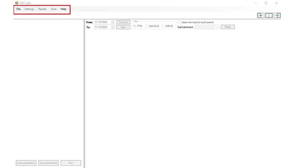
Upon opening HBV-light, it has 5 different tabs, including ‘File’, ‘Setting’, ‘Results’, 'Tool', and ‘Help’. Before importing the data, only the ‘File’ and ‘About’ tabs are active. ‘File’ tab contains ‘Open’ to open a project and ‘Exit’ to leave the software. ‘Help’ tab has ‘HBV-light help' which includes a guideline that how the software works and ‘About’ that gives detail about the software.
Fig. 4. HBV-light software environment showing the main tabs File, Setting, Results, Tools, and Help.
For importing our data, click on ‘Open’ in the ‘File’ tab, and then you should select the folder where both the ‘ptq’ and ‘EVAP’ files exist. After importing the data, other tabs in the software should be activated. ‘Setting’ has subtabs ‘Model settings’ and ‘Catchment Settings’, which are the important parts of the model for creating the basin information. ‘Results’ has one subtab that is ‘Summary’, which summarizes the results of the simulation by statistical metrics. ‘Tools’ tab has ‘Monte Carlo Runs’ , ‘Batch Runs', and ‘Gap Optimization'. These are useful for the calibration process.
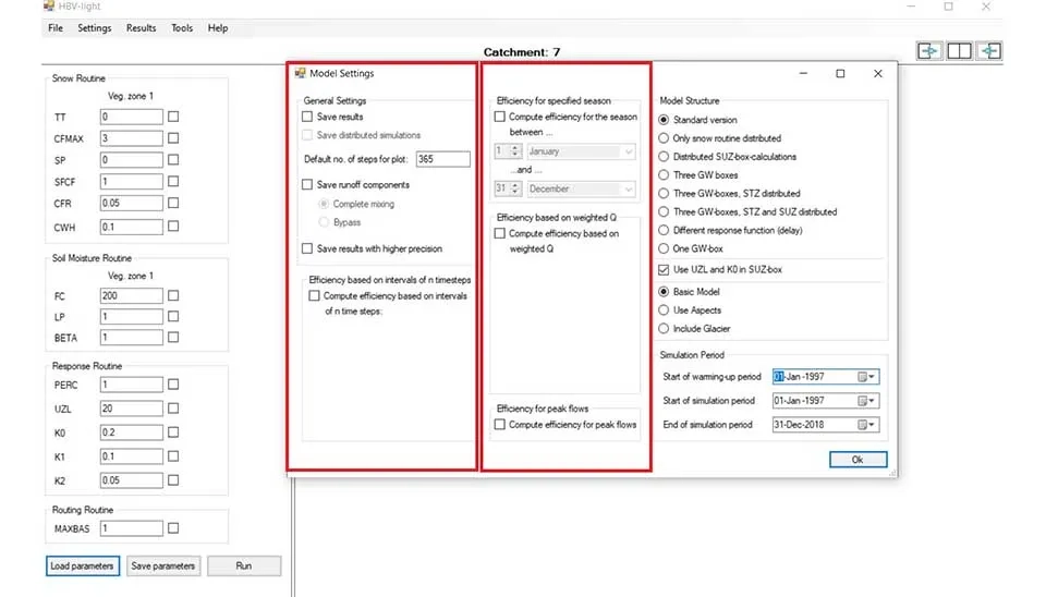
Model settings comprise different sections; first is a general setting that saves the results and distribution results and adjusts the step of the graph, or saves the run of components; For importing our data, click on ‘Open’ in the ‘File’ tab, and then you should select the folder where both the ‘ptq’ and ‘EVAP’ files exist. After importing the data, other tabs in the software should be activated. ‘Setting’ has subtabs ‘Model settings’ and ‘Catchment Settings’, which are the important parts of the model for creating the basin information. ‘Results’ has one subtab that is ‘Summary’, which summarizes the results of the simulation by statistical metrics. ‘Tools’ tab has ‘Monte Carlo Runs’ ,‘Batch Runs', and ‘Gap Optimization'. These are useful for the calibration process. Model settings comprise different sections; first is a general setting that saves the results and distribution results and adjusts the step of the graph, or saves the run of components; also you can save the result with higher precision among different runs. Under this section you can compute efficiency between the time steps in your simulation. In the center efficiency for a specific time or season can be calculated. Also you can weight the discharge and compute its efficiency , or just calculate this feature for pick discharge, which is useful for flood modeling and analysis.
Fig. 5. General settings and efficiency options in HBV-light software.
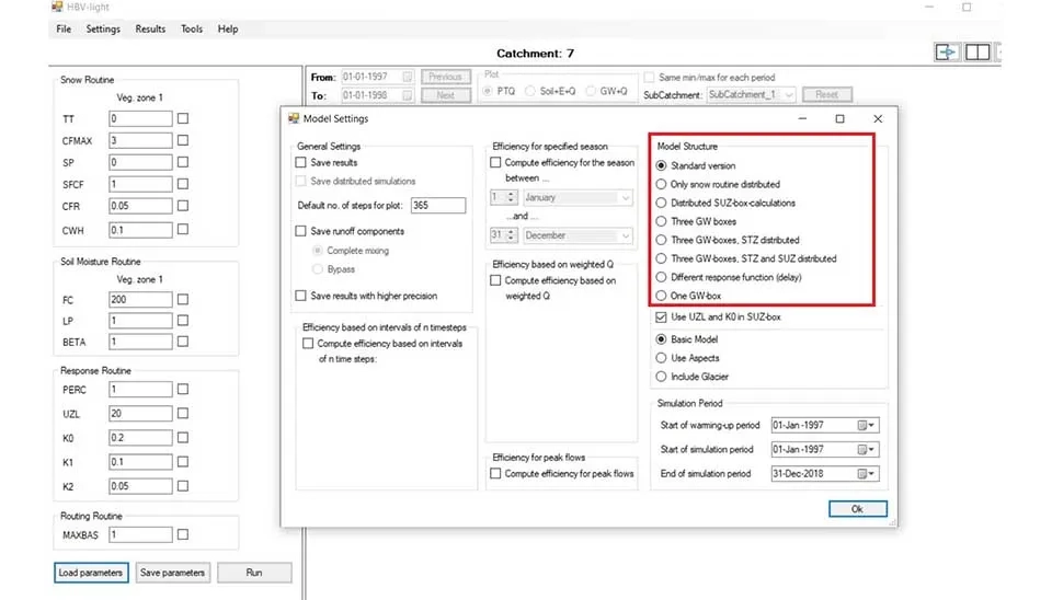
On the right, you can choose different model structures based on their spatial distribution. ‘Standard version’ assumes a lump approach for all parameters of the model, ignoring the spatial variability. ‘Only snow routine distributed' distributes only snow cover and snow accumulation spatially, assuming other parameters are lumped. ‘Distributed SUZ-box calculations’ divides the catchment based on SUZ (Soil Upland Zone), which is the upper soil layer where rapid infiltration and runoff occur, and assumes different values for each of them (Seibert 2005). ‘Three GW boxes’ separates the groundwater into three parts (shallow, intermediate, and deep groundwater layers) with separate storage volumes, giving detailed information about the groundwater variability. ‘Three GW Boxes, STZ distributed’ in this model you have 3 separate groundwater in addition to Store Zone (STZ) , which distributes in the model. STZ allows deeper storage zones, enabling spatial variability for groundwater.
You can save the result with higher precision among different runs. Under this section, you can compute efficiency between the time steps in your simulation. In the center, efficiency for a specific time or season can be calculated. Also, you can weight the discharge and compute its efficiency , or just calculate this feature for pick discharge, which is useful for flood modeling and analysis.
Fig. 6. Different model structures available in HBV-light software.
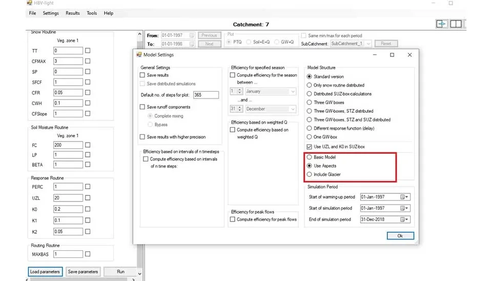
’Three GW boxes, STZ and SUZ distributed’ model incorporates the distribution of STZ ,SUZ , and groundwater across the catchment, allowing a more sophisticated structure with distribution of soil moisture and groundwater.’Different response functions (delay)’ model can vary the response function, which refers to how runoff and groundwater can delays. This model has a different response function for each component. ‘One GW box’ is a similar model that uses a single part of groundwater for the entire basin. For our modeling , we use ’Three GW boxes, STZ and SUZ distributed’ to get more detailed information about the hydrological process. There are three configurations in the model. ‘Basic Model’ includes only fundamental elements for hydrological modeling without considering spatial variability. The ‘Aspects’ model, which we use in our simulation, allows certain parameters to vary spatially across the catchment. The 'Include Glacier’ configuration is suitable for glacier-affected catchments where glacier mass, storage and coverage can be modeled.
Fig. 7. Different model configurations in HBV-light software.
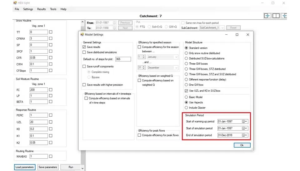
The last part is the simulation period, where you can specify the date for warming up and the start and end of the simulation. Warm up is a preliminary phase that allows the model to find the initial states of the parameters. If you have a long record of input data, you can use this option for 5 to 10 years. Because our data is limited, we don’t use this option and adjust 1 January 1997 to 31 December 2019 for simulation.
Fig. 8. Simulation period settings in HBV-light software.
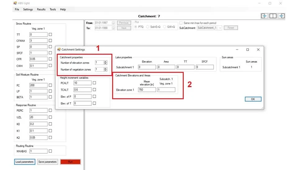
One of the important parts of the software is ‘Catchment Setting’ , which comprises different parts. In the catchment properties, you can divide the catchment into the different elevations and vegetation zones. If your study area varies significantly by elevation , different elevation zones can be used, and the value can be the mean of elevation in that particular proportion. Elevation zones are especially vital for snow melting calculation. Since our catchment elevation only changes from 900 to 600m, we use one elevation zone with a value of 750m. Different vegetation zones can also can be defined by specifying the value of each vegetation type on a specific zone. For example, 0.2 is in elevation zone 1 and 0.8 in elevation zone 1. We use one vegetation zone for our modeling.
Fig. 9. Defining elevation and vegetation zones in HBV-light's catchment settings.
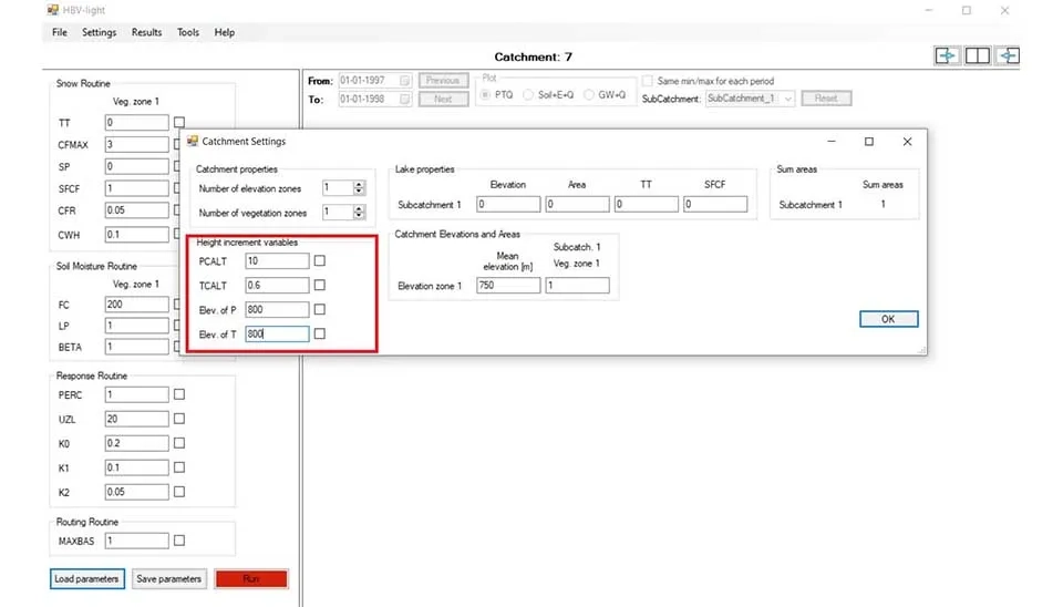
‘Height incremental variables’ is another component of ‘Catchment Setting’ , which helps to identify how precipitation and temperature changes by height. ‘PCALT’ is about how the precipitation varies by altitude, in general precipitation increases with increase in height. The ‘PCALT’ defined as the percentage increase in precipitation per 100 meter elevation and predefined values in 10 [%/100 m] is reasonable. ‘TCALT’ is the temperature change with altitude, defined as the decrease in temperature (°C) per 100 meter elevation. The value 0.6 is generally acceptable. 'Elev. of P' and 'Elev. of T' are the altitudes of the station where precipitation and temperature were derived. In our case it is 800m. The last part is ‘Lake properties’ ; you can define a lake in the model by the lake elevation, area (as a fraction of the sub catchment area), along with other variables.
Fig. 10. Height variables in HBV-light's catchment settings.
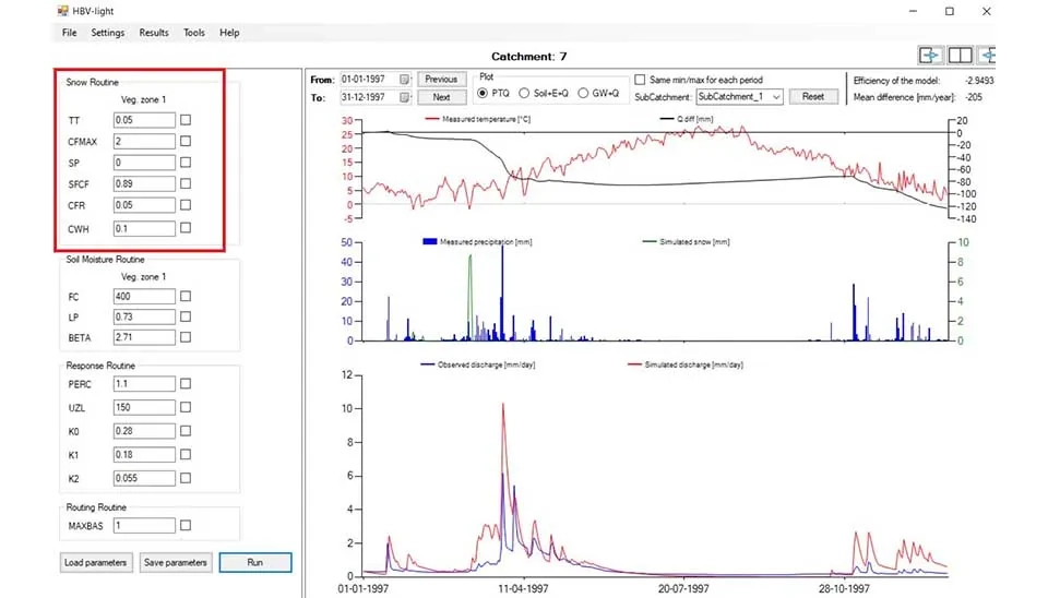
Moving to the main screen of the software, on the left different routines involving Snow routine , soil moisture routine and response routine can be seen. The snow process incorporates several essential parameters: TT (temperature threshold) specifies the temperature at which precipitation occurs as rain and below which it occurs as snow. CFMAX establishes the maximum snow accumulation capability, constraining the snow storage (assessed in mm of water equivalent). SP indicates the existing snowpack storage, which is revised according to precipitation and temperature (Girons Lopez et al. 2020). SFCF is a correction factor that modifies the snowfall accumulation to reflect regional and environmental influences. CFR, the degree-day factor, regulates the rate of snowmelt according to temperature, showing how much snow melts each day for every degree Celsius above freezing. Ultimately, CWH indicates the potential for extra snowmelt heat, taking into account external energy sources such as solar radiation or wind, which affect the snowmelt rate.
Fig. 11. Snow routine in HBV-light software.
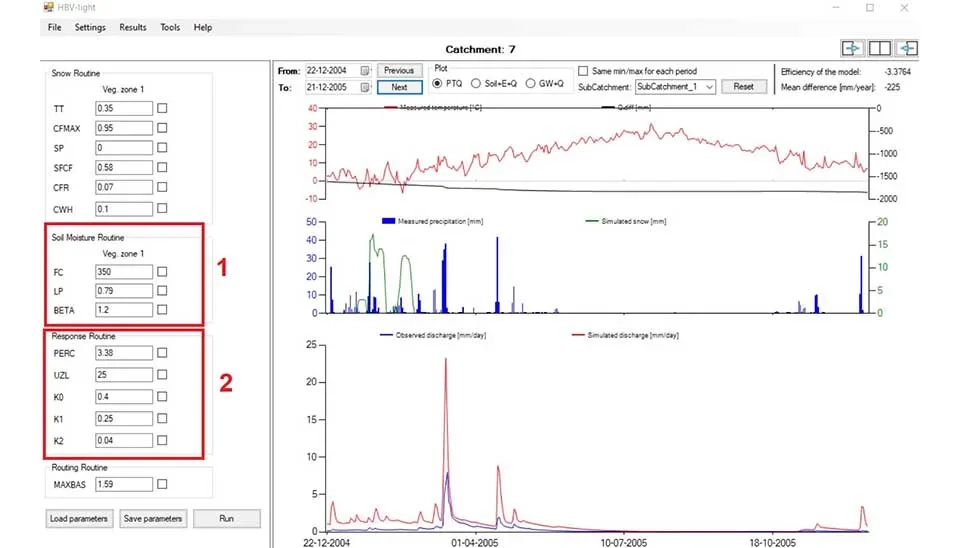
In the soil moisture routine FC (Field Capacity) shows the highest volume of water the soil can hold after surplus water has drained, denoting the moment when the soil is completely saturated but no infiltration happens. LC (Lower Limit of Soil Moisture) indicates the lowest moisture content, commonly referred to as the wilting point, beneath which plants struggle to effectively absorb water. Beta is an exponential factor that governs the speed of moisture release from the soil, affecting how rapidly soil dries out due to evaporation or percolation.
In the response routine, the percolation coefficient, PERC, regulates how quickly water decreases from the upper soil layer to deeper layers or groundwater. UZL denotes the upper zone storage, referring to the moisture retained in the active soil zone that leads to runoff during rainfall occurrences. K0 is a percolation rate constant that determines how quickly water travels from the upper zone to the lower zone, whereas KA manages the outflow of water from the upper zone into runoff, influencing surface discharge. K2 regulates the discharge from the lower region, signifying the input of baseflow or gradual groundwater release into streamflow. Collectively, these factors dictate the manner in which water is held, moves through the soil, and is discharged as runoff or baseflow, affecting both rapid and gradual hydrological reactions in the watershed.
Under the response routine the routing routine has only MXBAS, which indicates the highest storage parameter for baseflow. It specifies the greatest quantity of water that can be held in the baseflow storage (lower zone). The MXBAS parameter restricts the volume of water that can gather in the slower, deeper groundwater reservoir, which impacts the baseflow (the gradual runoff component) over time. When the baseflow storage hits this upper limit, no more water can be retained, and the surplus is either evaporated or discharged into the stream.
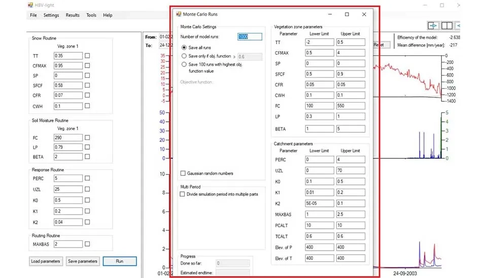
These parameters can be adjusted before the calibration process if you have prior knowledge about the study area or can be changed to the optimum values after the calibration step. After clicking ‘Run’ the hydrograph will appear on the main screen but it needs to be calibrated. From, ‘Tools’ tab , ‘Monte Carlo Run’ can be selected for calibration. Monte Carlo is a statistical method and a powerful tool for estimation of parameters by conducting numerous simulations with varying random sets of parameter values (Sammarah et al. 2023). In the software you can define a range for each parameter for calibration, an objective function and number of runs. You can define a variety of statistical metrics for objective function or even combination of them.
Fig. 13. Monte Carlo runs settings in HBV-light software.
There are a variety of choices for objective functions , such as coefficient of determination, Nash-Sutcliffe Efficiency (NSE), Kling-Gupta Efficiency (KGE) and also a Python script with a pre-process code. The results of the all simulation can be saved or a threshold for objective function can be defined to save the results. The results will be saved in text format in a folder where the input data exists, then the parameters can be transferred to the software manually.
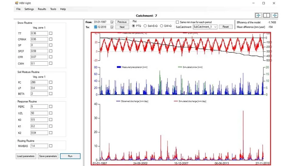
After running the software the graphs will appear on the main screen, and the results in a text file is available in the folder of the input dThe software offers three combinations of graphs ‘PTQ’ , ‘Soil+E+Q’ , and ‘GW+Q’. The first one has 3 graphs, measured temperature vs differential in discharge , measured precipitation vs simulated snow and most importantly simulations discharge vs observed discharge. The ‘Soil+E+Q’ offers the amount of water in the soil box , potential vs actual evapotranspiration, discharge vs observed discharge. ‘GW+Q’ offers upper groundwater accumulation , lower ground water accumulation, and simulations discharge vs observed discharge. The value of these variables also is available in the result file of the software for each time step. These graphs also can be used in manual calibration process.ata.
Fig. 14. Results of the simulation in HBV-light software.
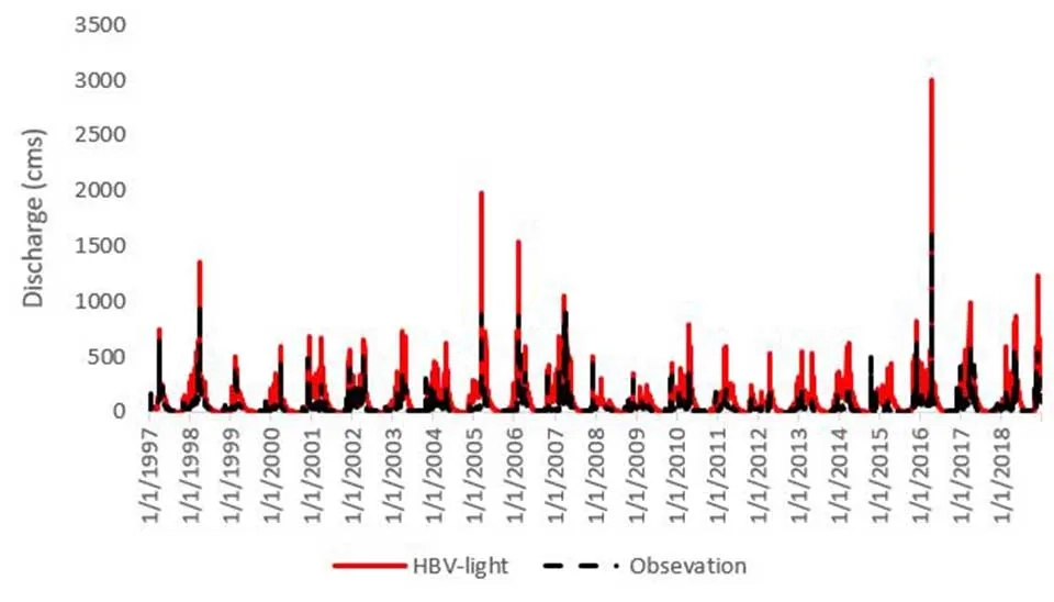
Throughout the simulated timeframe, HBV-light showed satisfactory results in modeling the hydrograph at the basin outlet, reaching a coefficient of determination (R²) of 0.82. This suggests that the model was able to account for around 82% of the observed fluctuations in daily streamflow, accurately representing the timing and scale of significant flow changes. Nonetheless, in spite of its general precision, the model encountered particular difficulties in replicating maximum flow scenarios. In particular, extreme flow events were frequently overestimated by different degrees, revealing notable differences between the simulated and real maximum flows. This miscalculation implies that the model might struggle to accurately depict intense rainfall occurrences or abrupt increases in runoff. For instance, 4/14/2016 where the observed flow was 1602 m3/s , the simulated flow by the model was 2905 m3/s, highlighting a massive error in this maximum flow Moreover, HBV-light consistently projected the base flow too high, resulting in a simulated streamflow that exceeded expectations during times of low rainfall. This pattern was especially apparent during the arid seasons, when river water flow reached its lowest points. In this situation, the model typically overpredicted streamflow, likely due to its assumptions about groundwater contributions or slow-recovery flow pathways.
Fig. 15. Comparison of observed and simulated discharge using HBV-light.
The full daily results are available in the CSV file via Results link.
5. Comparison between IHACRES and HBV-light
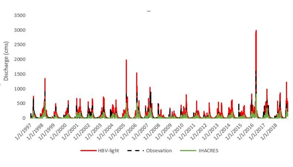
In another article ‘A Practical Guide to Using IHACRES for Hydrological Modeling‘, we introduce a comprehensive , step by step guide to the IHACRES model. The IHACRES model employs a straightforward design, functioning as a lumped model suitable for different climatic regions, including arid and semi-arid zones (Croke and Jakeman 2008). The main objective of the IHACRES model is to evaluate the hydrological behavior of the basin using a restricted number of parameters, including just precipitation and temperature. These 2 models are similar and have been used in different studies and we want to make a comparison between them. Both models depict overall satisfactory results and proved to be effective tools in hydrological modeling. HBV-light with coefficient of determination of 0.82 had better performance than IHACRES with R² of 0.744, indicating a better performance during the simulation period. However, both models struggled with simulation of maximum flows , while IHACRES underestimates them and HBV-light overestimates them. For example, in 4/4/2016 while the observed flow was 1602 m3/s , the IHACRES and HBV-light estimated it 823 m3/s and 1602 m3/s, respectively.Both models also have similar limitations in base flow simulation. IHACRES consistently overestimates base flow, especially during dry or low-rainfall periods, suggesting that it assumes too much groundwater contribution or slow recovery from earlier rainfall events. Similarly, HBV-light also over predicts base flow during arid seasons when the river’s flow is minimal, pointing to the model's tendency to assume higher groundwater contributions or slower response to low-flow conditions than actually occurs. In summary, while HBV-light slightly has better performance than IHACRES, with a higher R² value, both model share a same weaknesses, particularly in extreme flow events—underestimation by IHACRES and overestimation by HBV-light—as well as overestimation of base flow during dry periods.
Fig. 16. Comparison of observed and simulated discharge using IHACRES and HBV-light.
Hybrid approach is one effective tool that researchers employ to use the results of the different models and unite them, such as using multiple models and weight the results of them , or use the output of a model as an input to another model ( especially in case of using machine learning models). For instance, as observed, IHACRES tends to underestimate maximum flow events, while HBV-light tends to overestimate them. By averaging the two models, we can offset the error in maximum flow simulation, resulting in higher accuracy. However, the overestimation in base flow still persists. Because averaging the results of the two models would not address this specific flaw, as both models exhibit the same tendency to overestimate base flow in these conditions.
6. Conclusion
Hydrological modeling enables us to understand and simulate the response of a basin in precipitation. This becomes useful especially in climate change periods where events become extreme. In this article we delve into the step by step guideline of HBV-light software, a robust tool for hydrological modeling that needs minimum climatic data (precipitation, temperature, and evapotranspiration). The guideline included the function of HBV-light, how the input data structure should be, the different parameters and structural model , and calibration process. The results showed good accuracy of the HVB-light software, with a coefficient of determination (R²) of 0.82, indicating that the model effectively captures the variability in daily streamflow. Despite its strengths, the model demonstrated some limitations, particularly in simulating extreme flow events and base flow during dry periods. In addition to discussing the performance of HBV-light, the comparison with another hydrological model, IHACRES, was provided. While HBV-light demonstrated a higher coefficient of determination (R² = 0.82), indicating better overall accuracy, IHACRES (R² = 0.744) also showed solid performance, particularly in simulating regular flow dynamics. However, both models exhibited similar limitations when it came to extreme flow events and base flow simulation.
HBV-light for Hydrological Modeling: A Beginner's Guide | Waterlyst


Comments
No comments yet
Be the first to comment
Share your thoughts and start the conversation.