A Practical Guide to Using LARS-WG for Climate Data Downscaling

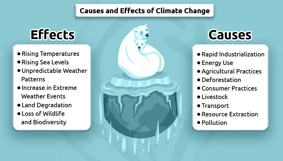
Imagine a world where predictable rainfall patterns have become unpredictable, where floods occur unexpectedly and droughts last longer than they ever have. This isn't a far future; it's the reality we confront now as climate change disturbs the fragile equilibrium of the water cycle, exacerbating water scarcity and severe climate incidents worldwide. The indicators from extreme heat to devastating floods show that our Earth is heating up at a concerning speed, and the moment to take action is now. Climate change is emerging fast as a significant concern for the 21st century due to its harmful effects on the environment and society. In the context of climate change, rapid shifts in the atmospheric system have heightened both time-related and spatial fluctuations in the water cycle and exacerbated water scarcity at both global and regional levels (Yang et al., 2021).

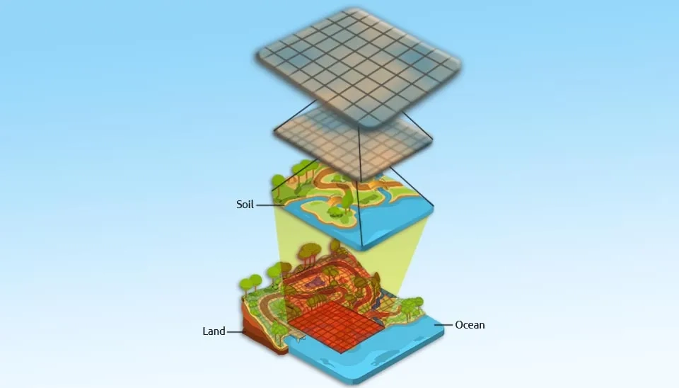
Climate change impact studies are crucial, and utilizing General Circulation Models (GCMs) is a productive way to achieve this. Nonetheless, GCMs generally provide a low spatial resolution, which restricts their capacity to represent climate processes at the watershed level—a vital element for localized climate impact research (Xu and Yang 2015). As a result, there is a need for downscaling techniques that refine GCM output on a regional scale, providing valuable inputs for localized impact assessments. One of the stochastic weather generators that has been proven to be reliable in identifying intricate patterns for the prediction of spatial-temporal data is the Long Ashton Research Station Weather Generator (LARS-WG) model, since it is less computationally expensive, easier to use, and demands fewer computer resources than dynamical downscaling strategies.

1. Why use CMIP6?

The IPCC (Intergovernmental Panel on Climate Change) is a nongovernmental agency founded in 1988 by the United Nations (UN) and the World Meteorological Organization (WMO). The Coupled Model Intercomparison Project (CMIP), initiated in 1995, is the IPCC’s project to develop Assessment Reports (ARs) on climate change. These reports outline what is known about climate change, its effects, and potential mitigation and adaptation strategies. 

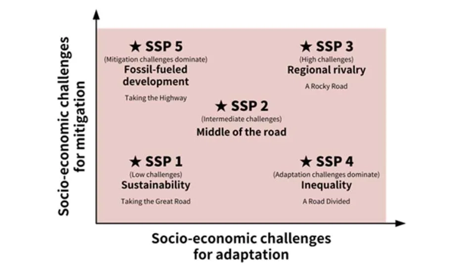
The latest CMIP is CMIP6, a notable enhancement that incorporates Shared Socioeconomic Pathways (SSPs), which offer various scenarios for potential future socioeconomic growth. These situations, spanning from sustainable low-emission routes (SSP126) to high-emission, fossil-fuel-reliant growth (SSP585), are combined with Representative Concentration Pathways (RCPs) to simulate varying degrees of radiative forcing by the year 2100 (Zarei et al. 2023).

GCMs play a vital role for exploring climate change and have been widely used to project precipitation patterns across the globe under different greenhouse gas scenarios. However, GCMs only provide coarse spatial resolution; therefore, they struggle to capture climate processes at a watershed scale, which is important for climate impact studies at the local level (Troin et al. 2015). Therefore, developing downscaling techniques is needed to refine the information from GCMs on a regional scale and provide useful inputs for local impact studies.

2. LARS-WG

The LARS-WG can be used to downscale the GCM outputs. The results can be used for water availability and agriculture analysis,  by analyzing rainfall patterns for crop growth. The LARS-WG generates daily solar radiation, temperatures (minimum and maximum), and precipitation at a particular site for future and current climate periods. The simulation of precipitation occurrence is modelled as an alternate wet and dry series, where a wet day is defined to be a day with precipitation > 0.0 mm. For precipitation calculation. It utilises semi-empirical distributions for the lengths of wet and dry day series, daily precipitation and daily solar radiation. For daily minimum and maximum temperatures are considered as stochastic processes with daily means and daily standard deviations conditioned on the wet or dry status of the day. The seasonal cycles of means and standard deviations are modelled by finite Fourier series of order 3 and the residuals are approximated by a normal distribution. For solar radiation, separate semi-empirical distributions are used to describe solar radiation on wet and dry days.

In 1990, the Assessment of Agricultural Risk Project in Hungary included the initial release of LARS-WG. Semenov et al. 1998 assessed and approved the LARS-WG model’s efficiency at eighteen meteorological stations across Europe, Asia, and the United States.

LARS-WG uses a first-order autoregressive process to model the daily temperatures. The daily maximum temperature (T_max​) and minimum temperature (T_min)​ are generated using the following formulas:

T_max (t)=μ_max+σ_max . (ρ_max . (T_max (t-1)) - μ_max)+ ∈_max (t)                                     (1)

  T_min  (t)=μ_min +σ_min . (ρ_min . (T_min (t-1)) - μ_min)+ ∈_min (t)                                    (2)

T_max (t) and T_min (t) are respectively the highest and lowest temperatures for day t. The average high and low temperatures are indicated by μ_max and μ_min, and their standard deviations are represented as σ_max and σ_min. The autoregressive values of high and low temperature are ρ_max and ρ_min, and they show that the current temperature is driven by the temperature of yesterday. The random variables ϵ_max and ϵ_min represent the residual errors for the maximum and minimum temperatures, respectively, and are described as Gaussian random variables, adding stochastic variability to the temperature predictions.

LARS-WG models precipitation as a Markov process, where the occurrence of rain on a given day depends on whether it rained on the previous day. The method is often broken down into two main steps:

Step 1: Modeling the occurrence of rain (0 or 1): Precipitation is treated as a binary variable (whether it rains or not). The probability of rain on day t given the rain status on the previous day is given by:

Where, P_rain​(t) represents the probability of rain on day t, which is influenced by the maximum temperature on the previous day, T_max(t−1). The relationship between these variables is modeled using regression coefficients β₀​ and β₁​, which are derived from historical data. These coefficients quantify the dependence of the probability of rainfall on the previous day's temperature, allowing the model to capture how past temperature conditions influence the likelihood of precipitation on subsequent days.

Similar to temperature and precipitation, other weather variables like wind speed and solar radiation are generated using stochastic processes that account for temporal correlations (e.g., lag-1 autocorrelation) and the statistical properties of historical data. Once the model is calibrated using historical data (e.g., temperature, precipitation, etc.), it can generate synthetic weather data for future periods. Climate projections (e.g., from General Circulation Models or Regional Climate Models) can be used to adjust the parameters of the LARS-WG model, enabling the simulation of future climate conditions under different emission scenarios.

3. Study Area

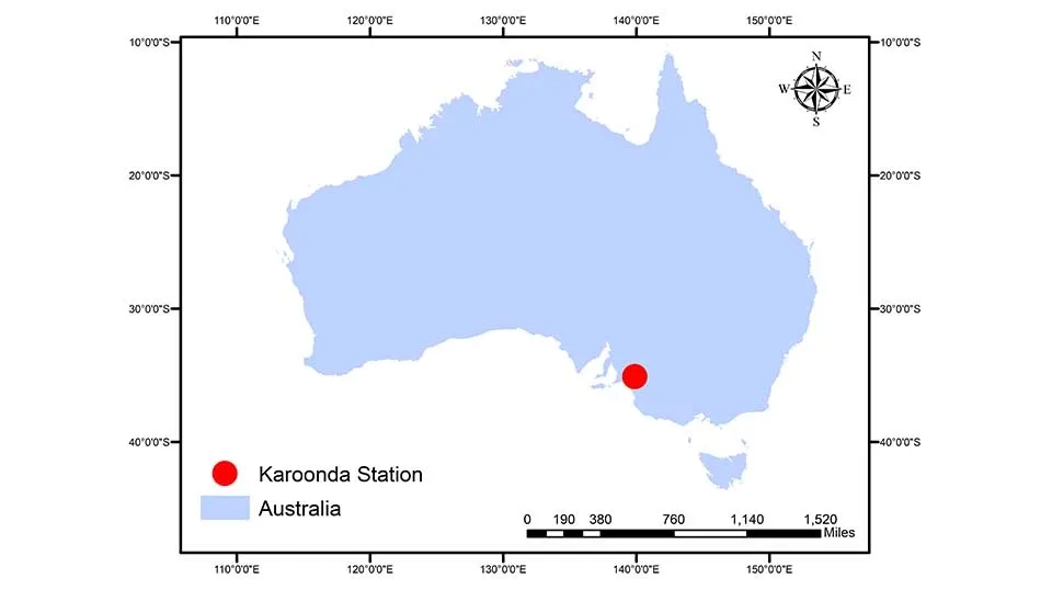
The Australian continent encompasses diverse climate zones, spanning from tropical areas in the north to dry inland regions and temperate climates in the south. The station selected for this study is located in Karoonda. This small region, situated in the Murray Mallee area of South Australia, usually has a semi-arid Mediterranean climate marked by hot, dry summer months and cool, wet winters. The typical yearly rainfall ranges from 300 to 350 mm, predominantly happening during winter and spring. Autumn is usually gentle and arid, marked by moderate temperatures. The region is mainly dedicated to agriculture, featuring significant cultivation of wheat, barley, oats, a few vineyards, and pastures reserved for grazing livestock. Natural vegetation is scarce, mainly comprising drought-tolerant species like mallee shrubs and saltbush. The region is appropriate for semi-arid climates, depending on irrigation for farming and managing water shortages during dry spells (Geoscience Australia). The station's coordinates are as follows: Latitude -35.09° (south) and Longitude 139.90° (east), with an elevation of 72 meters above mean sea level.

4. Dataset

4.1 LARS-WG 8

The latest version of LARS-WG is available at LARS-WG 8.0 for windows. It is important to note that the software's creators specify that LARS-WG can be used by individuals from academic, governmental, and non-profit organizations for research purposes. However, a license is required for use in funded research projects, and the software cannot be used for commercial applications. By using LARS-WG, users agree to share any derivatives, such as site parameters and diagnostic files. The software’s eighth version includes an update incorporating a limited selection of CMIP6 GCMs, marking a significant improvement over previous versions.

4.2 Observation data

LARS-WG requires daily climate data either precipitation (mm), maximum temperature (°C), minimum temperature (°C), and sunshine duration (hours/day) , or precipitation (mm), maximum temperature (°C), minimum temperature (°C), and solar radiation (MJ/m²). With these inputs, LARS-WG can make downscaled, high-resolution climate data, which is very important for figuring out how climate change affects places and how it affects regions as a whole.

4.3 Observation data pre-processing

We have used the available data from the Australian Bureau of Meteorology (http://www.bom.gov.au/climate/data/). After selecting the desired station, we downloaded the climatic data (daily precipitation, minimum and maximum temperature, and other relevant variables) in.csv format. It is important to note that the observation data should ideally span over a period of more than 10 years, though a longer dataset is preferred. For the selected station and available data, we used data from January 1, 2003, to December 31, 2014. Another important aspect is handling missing values. The LARS-WG software identifies missing values as -99, so in the CSV file, we replace the empty cells (missing values) with -99.

Table  1. First rows of the input data structure in Excel.

Note: For brevity, long terms are presented in abbreviated form as follows:

Abbreviations: Y= Year; M= Month; D= Day; Max T= Maximum Temperature; Min T= Minimum Temperature; P= Precipitation; SR= Solar Radiation.

The output information is extensive, so we only provide ten rows. For comprehensive information, engineers can refer to the table below:

The input data for LARS-WG must be in a DAT file (.dat). Based on our climatic data, we format the Excel columns into Year, Month, Day, Maximum Temperature, Minimum Temperature, Precipitation, and Radiation, without including headers in the CSV file. Then save the file as a DAT file (.dat) for use in LARS-WG. 

Table 2. First ten rows of the input data structure in the DAT file.

Note: For brevity, long terms are presented in abbreviated form as follows:

Abbreviations: Y= Year; M= Month; D= Day; Max T= Maximum Temperature; Min T= Minimum Temperature; P= Precipitation; SR= Solar Radiation.

For access to the whole data, you can use the following link.

5. Working with LARS-WG 8

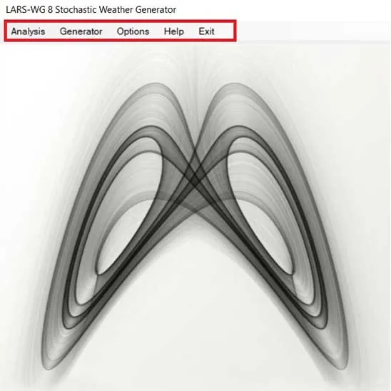
Upon opening LARS-WG, we encounter five different tabs: Analysis, Generator, Options, Help, and Exit. Analysis allows users to examine and analyze input climate data; Generator is used to generate weather data based on observed data for either historical or future periods based on the GCM; Options enable users to adjust software settings and change the location of input or output data; Help provides access to documentation and user guides; and Exit closes the program. These tabs facilitate the processes of analyzing, generating, and configuring climate data while offering support for users .

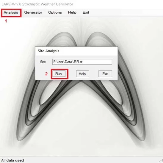
First, we work with the Analysis tab. After selecting our DAT file and clicking 'Run,' LARS-WG 8 will perform several statistical tests based on the observation data, which can give us comprehensive results about the performance of the software as well as information about the variability of our observed data.

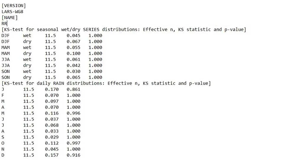
The software will provide statistical tests, such as the Kolmogorov–Smirnov (KS) test for seasonal wet/dry series distributions, the KS test for all climatic input data distributions, the monthly mean and standard deviation for all climatic input data, paired t-tests to detect biases for monthly means, and the KS test for all climatic input data distributions. 

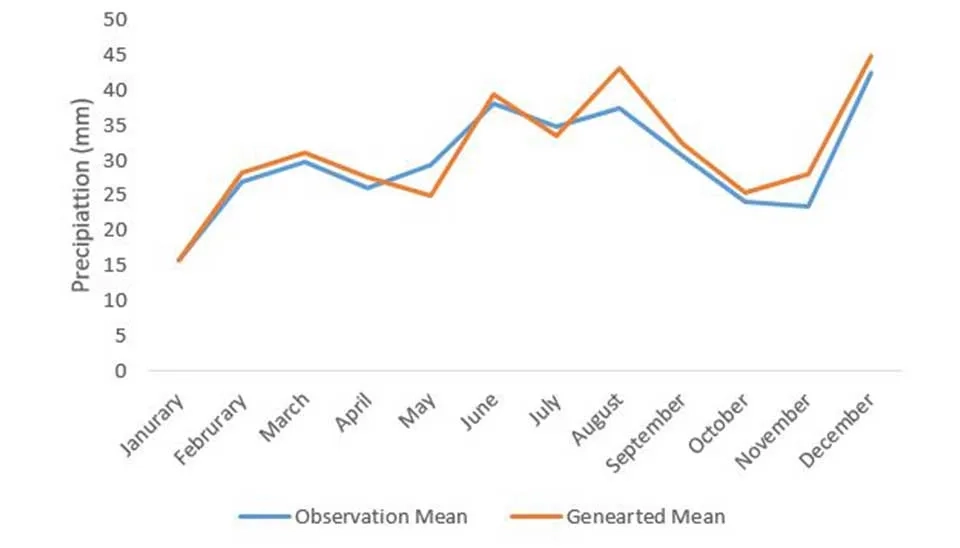
The comparison between the observed mean and generated mean values by LARS-WG8 reveals notable discrepancies in the model's performance. The generated mean closely tracks the observed mean for most months, but there are certain months where the model's performance varies significantly. For example, the generated mean overestimates the observed values in August (generated: 43.11, observed: 37.48) and December (generated: 44.93, observed: 42.43), while it underestimates values in May (generated: 24.89, observed: 29.43). The model is relatively accurate in January, February, and March, with small discrepancies, but June (generated: 39.39, observed: 38.06) and October (generated: 25.41, observed: 24.08) show close alignment. The R² value of 0.90 and RMSE of 2.74 mm highlight the model 's performance. Overall, these results suggest that the model performs reasonably well in replicating the general seasonal patterns. Thus , it can be used to fill the gap in the historical period.

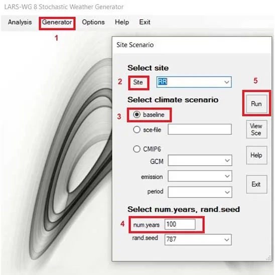
If the result is satisfactory , we navigate to the Generator tab. By selecting the baseline option and specifying the number of years, we can generate data for the historical period to fill in the gaps in our observation data. 

The results will be saved in the Output folder where the software is extracted. 

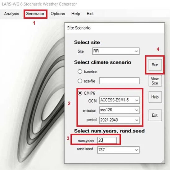
5.1. Downscaling when the most suitable GCM for the study area is already identified

If we already know the best GCM for our research area, for example, by reviewing other papers that focus on the same region of interest. We first select our observation file (.dat), followed by CMIP6. In the GCM section, we have a variety of models to choose from, including ACCESS-ESM1-5, BCC-CSM2-MR, CanESM5, CESM2, CMCC-ESM2, GFDL-ESM4, CNRM-CM6-1, GISS-E2-1-G, HadGEM3-GC31-LL, INM-CM5-0, MIROC6, MPI-ESM1-2-LR, MRI-ESM2-0, TaiESM1, and UKESM1-0-LL. Additionally, we can select from three emission scenarios: SSP126, SSP245, and SSP585, with data available for different periods ranging from 2021 to 2100.

For example, if we already know that ACCESS-ESM1-5 is the best model, we select it along with SSP126 and the period from 2031 to 2050. We then adjust the number of years (preferably matching the length of the observation data) and click 'Run.' 

The results will be saved in the Output folder. When extracting the data from the software, the first row will indicate the start year—January 1, 2031 in this case—and the order of the columns will match the input data from the initial .dat file.

Table 3. First rows of the results 

Note: For brevity, long terms are presented in abbreviated form as follows:

Abbreviations: Y= Year; M= Month; D= Day; Max T= Maximum Temperature; Min T= Minimum Temperature; P= Precipitation; SR= Solar Radiation.

For access to the whole data follow the link.

5.2. Downscaling when the most suitable GCM for the study area is unknown 

Since the raw GCM data is unavailable for a specific location through LARS-WG, we choose to download the raw data externally and import it into the software. There are several sources from which we can obtain GCM data, and two useful ones are Climate4Impact and Copernicus Climate Data Store. 

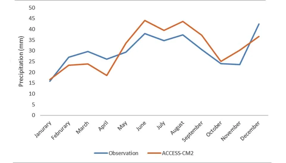
We typically need to download a large number of GCMs (more than 10) to evaluate their performance and select the most suitable one. GCMs have two main files: generated historical data and generated future projections. To find the best model, we only need to download the generated historical data from the GCM to assess its performance against our observational data. After finding the best GCMs we download their data for future projections. As a general note, projecting precipitation is more challenging than modeling temperature and radiation due to its inherent variabilities. Thus, precipitation should be the primary factor for choosing the GCM model if you intend to project  other variables. For instance, we downloaded historical precipitation data for ACCESS-CM2 for the historical period and compared it with our observational data.The analysis of the historical data in comparison with the results from the ACCESS-CM2 model shows varied performance of this GCM for the station. The ACCESS-CM2 model generally underestimates the recorded values for the majority of months, particularly between January and April, with significant differences in February (estimated: 23.28, observed: 27.04) and April (estimated: 18.55, observed: 26.12).  This is because of the low amount of precipitation in summer that most GCM models struggle to accurately capture. Nonetheless, it demonstrates improved alignment in the subsequent months, especially from May to December, with the estimated figures being nearer to the observation data, yet there remains some overestimation, particularly in June (estimation: 44.12, observed: 38.06) and August (estimation: 43.70, observed: 37.48). In spite of these differences, the R² value of 0.81 shows that the model accounts for 81% of the variation in the observed data, indicating a robust correlation between the estimated and actual values. The RMSE of 5.26 mm emphasizes that the model's predictions differ from the actual values by an average of 5.26 mm, which is a justifiable error margin given the data's scope. In summary, these findings indicate that ACCESS-CM2 is appropriate for reproducing historical climate records at this site; consequently, it can be utilized for future precipitation forecasts.

The precipitation, maximum and minimum temperature, and solar radiation data for the future period (2020–2100) from ACCESS-CM2 were downloaded to prepare the input data for LARS-WG8. 

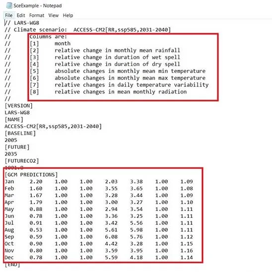
We need to prepare the input data as a .dat file, with the first column being the month's names. The second one is the relative change in monthly mean rainfall that is calculated as follows:

The third column is about the relative change in duration of the wet spell and the relative change in duration of the dry spell that are generally considered 1 for all months. Fourth and fifth columns are absolute changes in monthly mean minimum  temperature, and absolute changes in monthly mean maximum temperature, calculated as follows:

The seventh column represents relative changes in daily temperature variability, which can be considered as 1 for all months. Finally, the last column shows the relative changes in mean monthly radiation, calculated as:

After calculating all the columns, for better clarity, there are other optional fields to fill in, such as name, baseline, and future. This process should be repeated for different scenarios and future time frames. For example, one file for the 2030–2050 range, another for 2050–2070, and so on.

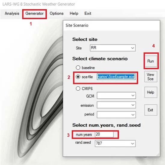
To use the scenario, go to the Generator tab, select the SCS file, adjust the number of years, and click "Run." The results will then be available in the output folder. The results of the simulation for the future period are in a text file where the first column is the first year of the future period (in our case , 2031) , the second column is the number of days in that respective year that ranged from 1 to 365, the third column is maximum temperature, the fourth is minimum temperature, and the fifth column is solar radiation.

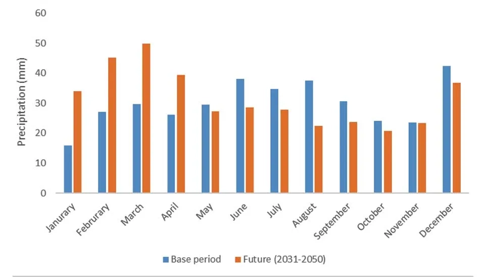
For educational purposes, we have modeled future precipitation based on SSP126 for the period of 2031-2050 based on ACCESS-CM2. The precipitation data from the reference period and future projections (2031-2050) derived from the ACCESS-CM climate model show significant changes linked to climate change and global warming. In January, the typical precipitation increases from 15.82 mm to 33.88 mm—an uplift of 18.06 mm or 114%. This suggests a rainier January and heightened flood risks that require adaptation and mitigation techniques. The February projection shows an increase from 27.04 mm to 45.21 mm, showing a rise of 18.17 mm (67%), which can affect early spring runoff and flood risks. In March, the measurement increased from 29.72 mm to 49.75 mm, indicating a notable increase of 20.03 mm (67%), potentially leading to increased soil saturation and surface runoff. In April, precipitation increased from 26.12 mm to 39.37 mm, a rise of 13.25 mm (51%), indicating wetter spring weather that could impact agricultural practices. Conversely, May projects a slight decrease of 2.10 mm (7%) from 29.43 mm to 27.33 mm. These figures in May suggest drought conditions. Summer months (June, July, and August) depict reductions—June declines from 38.06 mm to 28.58 mm, July from 34.76 mm to 27.86 mm, and August from 37.48 mm to 22.39 mm that account for 25%, 20% and 40% of reduction, respectively. These changes can lead to an exacerbation of water shortages and dryer summer seasons.  September shows a decrease from 30.61 mm to 23.70 mm (23%), indicating drier autumn weather that could hinder groundwater recharge and water resource management. Changes to irrigation and water conservation techniques might be essential. In October, precipitation decreased from 24.08 mm to 20.66 mm, indicating a reduction of 3.42 mm or 14%. The reduction in precipitation during autumn can greatly impact soil moisture and runoff patterns, especially in areas where these runoffs are crucial for restoring winter water supplies. In November, precipitation decreased marginally from 23.53 mm to 23.29 mm, indicating a small reduction of less than a millimeter (0.24 mm). In December, there is a noticeable reduction, as precipitation falls from 42.43 mm to 36.82 mm, indicating a decline of 5.61 mm or 13%. This winter's decrease in precipitation affects snowpack gathering in colder regions and may change the timing of spring runoff patterns. Inadequate winter rainfall could threaten water accessibility for farming and drinking purposes, especially in regions reliant on winter precipitation to sustain reservoir levels. In summary, the variations in precipitation trends during autumn and extending into winter highlight worries about the management of water resources, stressing the necessity for strategies to alleviate possible effects on agriculture, ecosystem vitality, and human water usage as the seasons evolve. The results of the downscaling are available via this link.

6. Conclusion

In a time characterized by extraordinary environmental changes, thoroughly evaluating the impacts of climate change has turned into a critical issue.  One of the ways to study the impact of climate change is using GCMs and thus these models are coarse; we need to downscale them. Among the relatively wide range of downscale methods , LARS-WG , a weather generator, is a popular method that gains the attention of researchers due to its speed and simplicity. This article offers a comprehensive guide  for using the  latest version of LARS-WG for downscaling climate variables by using GCM CMIP6. A station located in Australia was considered for the purpose of downscaling. After a step-by-step guide into the LARS-WG8 that offers a comprehensive guide, precipitation values were projected for the mentioned station for the period of 2031-2050 under SSP126 by ACCESS-CM2. The  result showed that winter months will experience increased precipitation compared to the base period , but other months will remain unchanged or experience a decline in precipitation.