Previously, runoff modeling was really challenging and time-consuming, relying on complex formulas and manual calculations. Traditional methods required extensive expertise and often oversimplified natural systems. Runoff Modeling with Random Forest has become a powerful approach in hydrology, offering improved prediction accuracy compared to traditional methods. Today, artificial intelligence has transformed this field by enabling faster and more accurate modeling. AI techniques like machine learning analyze vast data sets, adapt to complex systems, and integrate diverse data sources for precise predictions. This advancement has made runoff modeling more efficient in water resource management, especially in urban areas.
Flooding is a significant environmental hazard that leads to severe economic and social repercussions. The impacts of floods are influenced by socio-economic conditions, infrastructure, and local environmental factors. Understanding these elements is crucial for effective flood management (Negi et al., 2022).Beyond immediate impacts, long-term recovery, and resilience strategies addressing socio-economic vulnerabilities are essential (Lapietra et al. 2022).
Machine learning models greatly improve runoff prediction using advanced algorithms and data-centric methods. These models incorporate historical data and atmospheric variables, enhancing forecasting accuracy, which is crucial for water resource management and flood mitigation. Accurate runoff prediction aids proactive planning and resource allocation and minimizes risks. Improved runoff forecasts contribute to early warning systems and comprehensive flood prevention strategies, reducing flood impacts and protecting communities (Yuyan Fan et al., 2024).
Fig. 1. Runoff Modeling with Random Forest: Visual guide showing a watershed and data analysis dashboard.
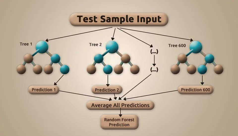
A Random Forest (RF) model, an ensemble learning technique for classification and regression, combines multiple decision trees trained on bootstrapped data subsets to produce robust results. This ensemble approach enhances accuracy, reduces overfitting, and provides resilience against data variability (
This document introduces the Random Forest model and its Python implementation, focusing on runoff estimation for a station in Canada. The study aims to evaluate the model's performance in hydrological prediction. The methodology, data analysis, implementation, and evaluation are discussed, concluding with insights into results. This guide provides readers with theoretical and practical knowledge of using the Random Forest model for hydrological studies.
1. Study area for Runoff Modeling
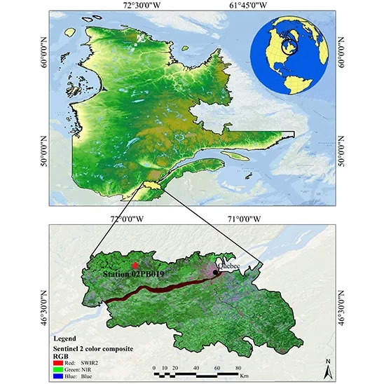
The study area is located between latitudes 46° 04′ N and 46° 59′ N and longitudes 72° 23′ W and 72° 30′ W, covering parts of four administrative regions in Quebec, Canada. It includes sections of Capitale-Nationale, Center-du-Québec, Mauricie, and Chaudière-Appalaches. The area lies within the Lower Saint Lawrence Basin, with the Saint Lawrence River running through it. The average elevation is 192 meters above sea level, with a maximum height of 688 meters. This region was selected for its fertile soils and growing coastal population.
Monthly runoff data from 2001 to 2013 were obtained from station 02PB 019 in this region (Soltani et al., 2021).
Fig. 2. Detailed map of the research site in Quebec, Canada, utilized for Random Forest runoff modeling.
2. Data Information
The data file contains valuable environmental and hydrological data that can support scientific research and management analyses of natural resources and ecosystems. Key columns such as distance from stream and elevation enable the examination of how proximity to water sources and land elevation influence vegetation cover and soil types in the region. Additionally, the Land Cover and Lithology columns offer insights into surface characteristics and the geological composition beneath, which are crucial for understanding the geographical and geological features of the area.
Moreover, the Normalized Difference Vegetation Index (NDVI) is an essential metric for evaluating vegetation health and density. Data on precipitation (Pr) and Runoff are invaluable for analyzing hydrological trends and informing water management strategies. By including month and year information, this dataset facilitates the study of seasonal and annual variations, enhancing environmental planning and water management. The data, spanning from 2001 to 2013, forms the basis for this study, which seeks to predict runoff using these variables:
In this section, we provide a comprehensive introduction to the Random Forest model as applied to runoff modeling, a powerful machine learning algorithm widely used for predictive analysis in hydrology. Along with a detailed explanation of the methodology, we break down and analyze the essential Python codes required for runoff modeling. This includes data preprocessing, feature selection, model training, evaluation, and visualization of results. The aim is to offer readers a clear understanding of how to implement and apply the Random Forest algorithm for hydrological modeling and runoff prediction effectively.
Fig. 3. Random Forest algorithm structure showing the aggregation of predictions from multiple decision trees.
3.1. Libraries
First, we import the necessary libraries, each providing a specific functionality. Data analysis and tabular data manipulation are done with the Pandas library. Numpy is a powerful tool for numerical computations and working with arrays and matrices. Matplotlib helps in creating charts and data visualizations. Seaborn, built on top of Matplotlib, provides additional capabilities for visualizing statistical data. Scikit-learn includes tools and algorithms for machine learning, such as data preprocessing and model training.
import pandas as pd
import numpy as np
import matplotlib.pyplot as plt
import seaborn as sns
import sklearn
The train_test_split function is used to split data into training and testing sets. labelEncoder is employed to convert categorical features into numerical values. RandomForestRegressor is a regression algorithm based on decision trees and is used for predicting numerical values. The metrics module contains functions for evaluating the performance of machine learning models, and PolynomialFeatures allows for expanding input features into polynomial representations.
from sklearn.model_selection import train_test_split
from sklearn.preprocessing import LabelEncoder
from sklearn.ensemble import RandomForestRegressor
from sklearn.metrics importfrom sklearn.preprocessing import PolynomialFeatures
3.2. Recall Dataset
The code begins by importing an Excel file named "ravanab.xlsx" using the Pandas library function pd.read_excel(). Here, the variable data is created to store the file contents as a DataFrame, which is a powerful data structure for handling tabular data, with rows and columns that make it easy to manipulate and analyze. This initial setup allows us to explore, clean, and preprocess the data effectively, preparing it for further steps in. It’s essential to ensure the file path is accurate, as any mismatch will trigger an error when attempting to load the file. With data properly loaded, we can access specific columns, make transformations, and extract features and labels necessary to feed into the Random Forest algorithm for building and testing the model.
data=pd.read_excel("/content/ravanab.xlsx")
3.3. Check the Dataset
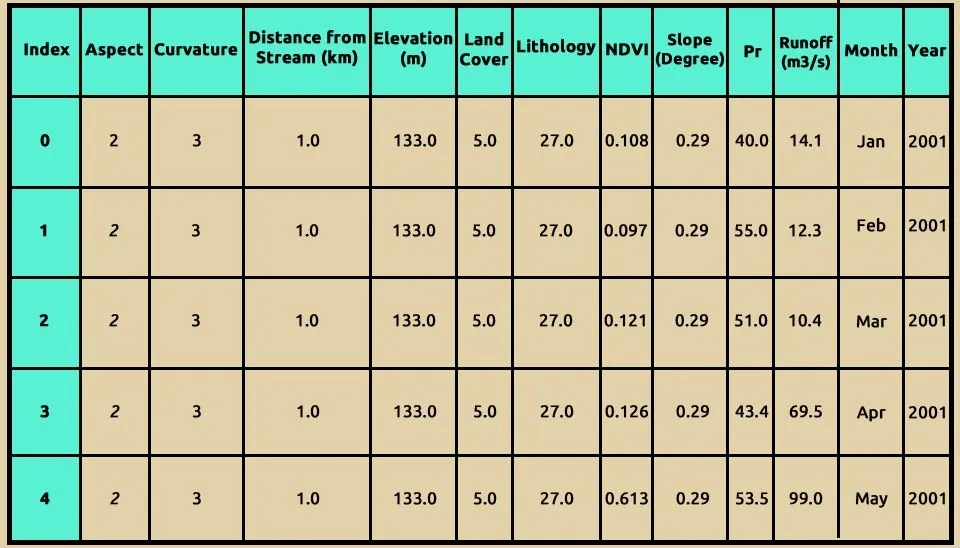
To better understand the dataset used for runoff modeling, the data.head() function in Python was employed to display the first five rows of the data. This preliminary step revealed key variables essential for predicting runoff, including distance from stream, elevation, land cover, lithology, vegetation index (NDVI), slope, precipitation, and runoff. These features are critical for understanding the physical and environmental factors influencing hydrological processes. Additionally, temporal information (month and year) was included to capture seasonal and annual variations in runoff. The dataset serves as the foundation for training and evaluating the Random Forest model, ensuring a comprehensive analysis of factors affecting runoff dynamics.
data.head()
Table. 1. Performance metrics of the Random Forest Model for Runoff Prediction during training and testing stages.
3.4. Check missing value and data type
The data.info() command provides a summary of our dataset. According to the displayed information, there are no missing values. However, the "Month" column is currently stored as an object data type. To utilize it effectively as a parameter, it should be converted to a numerical format.
data.info()
<class 'pandas.core.frame.DataFrame'>
RangeIndex: 156 entries, 0 to 155
Data columns (total 12 columns):
# Column Non-Null Count Dtype
--- ------ -------------- -----
0 Aspect 156 non-null int64
1 Curvature 156 non-null int64
2 Distance_from_stream(km) 156 non-null int64
3 Elevation(m) 156 non-null int64
4 Land Cover 156 non-null int64
5 Lithology 156 non-null int64
6 NDVI 156 non-null float64
7 Slope(Degree) 156 non-null float64
8 Pr 156 non-null float64
9 Runoff(m3/s) 156 non-null float64
10 Month 156 non-null object
11 Year 156 non-null int64
dtypes: float64(4), int64(7), object(1)
memory usage: 14.8+ KB
The dataset consists of 156 entries and 12 columns, with 11 numeric columns (float64) and (int64) and 1 categorical column (Month) of object type. All columns contain 156 non-null values, indicating a complete dataset with no missing entries, which is ideal for analysis and modeling. Key features such as Distance_from_stream(km), Elevation(m), Land Cover, Lithology, NDVI, Slope (Degree), and Pr (precipitation) represent environmental and physical factors influencing runoff.
The target variable, Runoff (m³/s), measures water discharge and is crucial for predictive modeling. Temporal columns like Month and Year add seasonal and annual context, which can help identify trends or patterns in runoff. The dataset’s small memory footprint (12.3 KB) makes it computationally efficient for machine learning applications. Overall, this clean and well-structured dataset is ready for exploratory data analysis, feature engineering, and machine learning tasks.
3.5. Changing the Data Type of The Month Column to Numerical Values
We utilize the LabelEncoder class from the sklearn.preprocessing module to convert the "Month" column in our dataset into a numerical format. This transformation is essential for many machine learning algorithms, which require numerical input rather than categorical data. The LabelEncoder is a utility class designed to normalize labels so that they contain only values between 0 and n_classes -1.
Table. 2. Dataset sample showing the categorical "Month" feature converted to integer values using LabelEncoder
3.6. Remove Same Feature
Since we have analyzed the data from one of the ten stations, certain features such as 'Aspect', 'curvature','Distance_from_stream(km)', 'Elevation(m)', 'Land Cover', 'Lithology', and 'Slope(Degree)' have identical values across all column. These features do not contribute to the model and are unnecessary for our analysis. To reduce computational complexity, we will remove these features. By using inplace=True, the specified columns will be permanently removed from the DataFrame, and the changes will be applied directly to the original DataFrame
data .drop(columns=["Aspect","Curvature","Distance_from_stream(km)", "Elevation(m)", "Land Cover", "Lithology",'Slope(Degree)'], inplace=True)
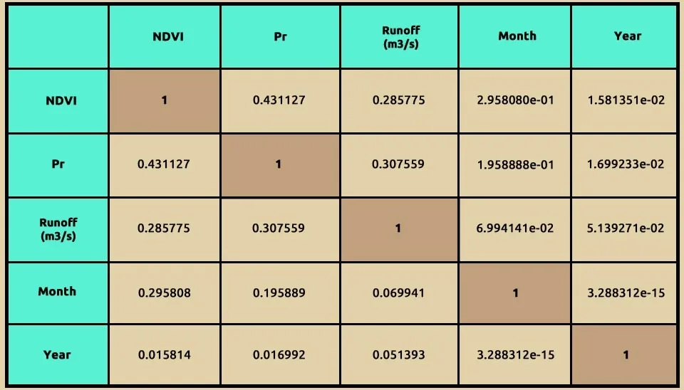
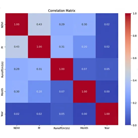
A correlation matrix is a table that shows the correlation coefficients between many variables. Each cell in the table displays the correlation between two variables, ranging from -1 to 1.
In python , you can easily compute a correlation matrix using pandas . here's how to compute and visualize the correlation matrix using a dataframe
Table. 3. Correlation Matrix for Random Forest Features, confirming Precipitation (Pr) has the strongest link to Runoff.
3.7. Show Correlation Matrix
This code generates a heatmap to visualize the correlation matrix of the dataset, helping to identify the strength and direction of linear relationships between variables. plt.figure(figsize=(10, 8)) creates a new figure with a specified size of 10 inches wide and 8 inches tall. The figure size is set to 10x8 inches for better readability. Adjusting the figure size ensures that the heatmap is legible and properly scaled for analysis or presentation.
sns.heatmap() function from the Seaborn library is used to generate a heatmap, which visualizes the correlation matrix.
Using Seaborn's heatmap function, the correlation coefficients are displayed on the heatmap cells (annot=True) with values formatted to two decimal places (fmt=".2f"). The cool warm colormap highlights positive correlations with warmer tones (red) and negative correlations with cooler tones (blue), making patterns visually distinct. A title, "Correlation Matrix," is added for clarity, providing an intuitive and detailed overview of the variable interactions in the dataset.
Fig. 4. Heatmap showing the variable correlations (ranging from -1 to 1) used in the Random Forest runoff modeling analysis
This heatmap visualizes the correlation matrix for the dataset, showing the relationships between variables. Each cell represents the correlation coefficient between two variables, ranging from -1 (perfect negative correlation) to +1 (perfect positive correlation). The diagonal cells show a perfect correlation of 1.0, as each variable is fully correlated with itself. NDVI and Precipitation (Pr) have a moderate positive correlation (0.43), suggesting that areas with higher vegetation (NDVI) may experience slightly higher precipitation. Runoff (m³/s) has a weak positive correlation with NDVI (0.29) and Precipitation (0.31), indicating that these factors influence runoff but not strongly. Temporal variables like Month and Year show minimal correlation with the physical variables, reflecting their independence in this dataset. The color scheme (coolwarm) highlights strong correlations in red and weaker ones in blue, making patterns and relationships visually distinct. This heatmap helps identify which variables are closely related and which may independently contribute to the runoff prediction model.
3.8. Selection Target Values and Features in The Form X and Y
target variable (y): this is the variable you are trying to predict. In this case , it's the Runoff
feature (x): these are the columns of the dataset that will be used to make predictions. To drop the Runoff column and use all the other columns as features.
X = data.drop(columns=['Runoff(m3/s)'])y = data['Runoff(m3/s)']
3.9. Splitting Data for Model Training and Testing
The train_test_split function from sklearn.model_selection is used to split a data set into two subsets: one for training model and two for testing . x and y feature and target data to be split .
test_size : an optional parameter that can specify the proportion of data to use for training.
random state: controls the shuffling of data before splitting . it ensures reproducibility of the split when set to an integer.
This shows that 80% of the data was allocated to training, and 20% was allocated to testing, based on the test_size=0.2 parameter.This will result in 124 samples for training and 32 samples for testing, exactly as you specified.
X_train, X_test, y_train, y_test = train_test_split(X, y, test_size=0.2, random_state=42)
3.10. Import Random Forest Regressor and Hyperparameter Tuning to Achieve the Best Model Performance Using GridSearchCV
Random forests are a combination machine learning algorithm. Which are combined with a series of tree classifiers, each tree casts a unit vote for the most popular class, then combining these results get the final sort result. RF possesses high classification accuracy, tolerates outliers and noise well and never gets overfitting (Liu et al., 2024).
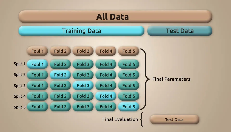
To achieve the best model performance, we perform model tuning using GridSearchCV to optimize key hyperparameters. In this case, a RandomForestRegressor is used with a parameter grid that includes variations in the number of estimators (n_estimators), the maximum depth of the trees (max_depth), and the minimum number of samples required to split an internal node (min_samples_split). The GridSearchCV is applied with 5-fold cross-validation to find the optimal.In the basic approach, called k-fold CV, the training set is split into k smaller sets (other approaches are described below, but generally follow the same principles). The following procedure is followed for each of the k “folds”
The performance measure reported by k-fold cross-validation is then the average of the values computed in the loop. This approach can be computationally expensive, but does not waste too much data (as is the case when fixing an arbitrary validation set), which is a major advantage in problems such as inverse inference where the number of samples is very small.
Fig. 5. Flowchart detailing the five-fold cross-validation process used by GridSearchCV to tune the Random Forest model.
The param_grid value is a dictionary in which a list of different values is defined for each model parameter to be used in the grid search process. In effect, param_grid tells the model what parameter values to try to find the best combination of them to optimize the model.
n_estimators: this parameter controls the number of trees in the random forest. More trees typically lead to better models but can also increase computational cost. The list [10, 50, 100] means that in the grid search process, three different values for the number of trees are tried: 10 trees, 50 trees, and 100 trees.
max_depth: this defines the maximum depth of the trees in the forest. Limiting the depth can help avoid overfitting. The list [None, 10, 20, 30] means that the model should be tested with four different values for the depth of the trees.
min_sample_split: This controls the minimum number of samples required to split an internal node . Larger values can prevent overfitting by forcing splits only when there are enough data points. 2 means that the split can be done with at least 2 samples (trees grow faster). 5 and 10 are more restrictive, and the model can consider more depth for larger data.
To calculate the predictions of the model on the test data (which the model has not seen) and the training data to check the accuracy of the model, evaluate the learning rate, and discover any possibility of overfitting or underfitting, in this section we use the X_test and X_train data to give our model. For the test data , the output of the prediction result is stored in the y_pred_test variable , and the predicted outputs for the training data are stored in the y_pred_train variable.
The model summary function evaluates the performance of the trained model by calculating and displaying key regression metrics for both the training and testing datasets. It takes as input the actual target values (y_train and y_test) and the predicted values (y_pred_train and y_pred_test).
The function first calculates the root mean squared error (RMSE) by taking the square root of MSE for a more interpretable error value. Also, it calculates the R-squared (R2) score, which indicates how well the model explains the variability of the target variable.
The function then prints these metrics for both the training and testing sets, allowing for clear comparison. The RMSE helps understand the average magnitude of error in the predictions , while the R2 score shows the proportion of the variance captured by the model , with values closer to 1 signifying better performance. This summary helps determine whether the model is overfitting, underfitting, or performing as expected on unseen data.
Based on these results, the model performs reasonably well but shows a slight drop in performance when moving from the training set to the testing set. For the training set, the RMSE of 17.4455 indicates the average prediction error, while the R2 score of 0.7852 suggests that the model explains approximately 78.52% of the variance in the training data. This indicates excellent predictive capability during training.
For the testing set, the RMSE is slightly higher at 19.149, showing that the model’s predictions have a larger average error on unseen data. The R2 score of 0.6795 implies that the model explains about 67.95% of the variance in the test data.
According to the results, the model shows excellent performance.
3.11. Adding Polynomial Features to Train and Test dataset
In machine learning , we can use polynomial features so that the model can learn more complex and non-linear relationships between features and the target variable . In simple linear models , the relationship between inputs and outputs is assumed to be linear , but in many real-world problems , this assumption may not be sufficient and more complex relationships exist.
By adding polynomial features, the model can learn nonlinear relationships that involve powers of features or interactions between them . For example, if an input sample is two-dimensional and of the form [a, b], the degree-2 polynomial features are [1, a, b, a2, ab, b2]. This expanded feature set enables the model to learn more complex patterns beyond linear relationships, enhancing its predictive capabilities.
degree : in this case , we create polynomial feature up to degree 4
interaction_only: by setting the interaction_only feature equal to false , in addition to the multiplicative feature , the individual powers of each feature are also considered.
The results indicate that adding polynomial features did not significantly impact the model's performance.
For the testing set, the RMSE increased slightly from 19.149 to 19.6626, and the R2 score saw a slight improvement from 0.6795 to 0.6899. However, these changes do not indicate a substantial improvement in generalization or predictive power.
3.12. Scatter Plots
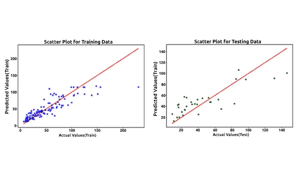
This code creates scatter plots to visualize the relationship between actual and predicted values for both training and testing datasets. First, a figure with two horizontally aligned subplots (1×2) is created, with an overall size of 20x7 inches. In the first subplot, the scatter plot for the training data is generated, where actual values (y_train) are plotted against predicted values (y_pred_train) using blue markers with an alpha value of 0.5 for transparency. A red dashed line represents the ideal relationship (perfect prediction), defined by the diagonal between the minimum and maximum values of y_train. Labels for the x-axis and y-axis are set as "Actual Values (Train)" and "Predicted Values (Train)," respectively, and the title is set to "Scatter Plot for Training Data."
In the second subplot, the scatter plot for testing data is drawn in a similar manner, with actual values (y_test) plotted against predicted values (y_pred_test) using green markers. Again, a red dashed line shows the ideal diagonal, and the axes are labeled as "Actual Values (Test)" and "Predicted Values (Test)," with the title "Scatter Plot for Testing Data." Finally, plt.tight_layout() ensures proper spacing between the subplots, and plt.show() displays the plots. This visualization helps assess how well the model's predictions align with actual values in both datasets.
These scatter plots illustrate the performance of a Random Forest model in predicting runoff data, with the left plot showing results for the training dataset and the right for the testing dataset. The red dashed line represents the 1:1 line where predicted values perfectly match actual values. The training plot demonstrates a strong correlation between predicted and actual values, as most points cluster near the red line, indicating excellent model fitting and high accuracy during training. In the testing plot, while the predictions still follow the general trend of the actual values, there is noticeable dispersion, especially at higher runoff values, suggesting slightly reduced predictive accuracy. The wider scatter in the test data compared to the train data may indicate overfitting, where the model performs better on training data than unseen data. The performance on test data shows some underestimation and overestimation at extreme values, which could be due to the variability in runoff or the complexity of the process being modeled. Outliers are present, particularly in the test set, where some points deviate significantly from the red line, suggesting that these cases might involve conditions not well captured by the training data. The Random Forest model appears effective overall, but its predictive performance could be improved by fine-tuning hyperparameters or addressing potential issues in the data. The high concentration of points near the red line in the training plot indicates the model's capacity to learn complex relationships in the data. A comparison of the plots highlights the importance of testing data to evaluate generalizability and avoid misleading conclusions based solely on training performance. Adding more features or improving feature engineering may help the model better capture the variability seen in the test set.
Fig. 6. Scatter plots comparing the predicted vs. actual runoff values for the training (left) and testing (right) datasets.
3.13. Comparison of Actual and Predicted Runoff
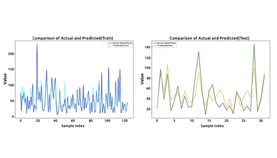
By plotting the actual and predicted values side-by-side, this visualization effectively highlights the model's performance, allowing for the identification of discrepancies such as overfitting, where the model achieves high accuracy on training data but performs poorly on testing data, or underfitting, where the model demonstrates inadequate accuracy on both datasets. This side-by-side comparison is crucial for assessing the model's reliability and robustness in runoff prediction. Below is the code used for visualizing the most recent training and testing data:
The line fig, axes = plt.subplots(1, 2, figsize=(20, 7)) is part of the Matplotlib library and is used to create a figure with two side-by-side subplots.
fig, axes = plt.subplots(1, 2, figsize=(20, 7))
This code generates a line plot on the first subplot (axes[0]) comparing the actual (y_train, in blue) and predicted (y_pred_train, in cyan) values for the training dataset. It includes labels for the x-axis ("Sample Index") and y-axis ("Value"), along with a title ("Comparison of Actual and Predicted (Train)"). A legend is added to differentiate between actual and predicted values, ensuring clarity.
axes[0].plot(range(len(y_train)), y_train, label='Actual Values (Train)', color='blue')
axes[0].plot(range(len(y_pred_train)), y_pred_train, label='Predicted (Train)', color='cyan', alpha=0.7)
axes[0].set_xlabel('Sample Index')
axes[0].set_ylabel('Value')
axes[0].set_title('Comparison of Actual and Predicted (Train)')
axes[0].legend()
This code creates a line plot on the second subplot (axes[1]) to compare actual (y_test, in green) and predicted (y_pred_test, in orange) values for the testing dataset. It includes x-axis ("Sample Index") and y-axis ("Value") labels, along with the title "Comparison of Actual and Predicted (Test)." A legend is added to distinguish between the actual and predicted values for better interpretation.
axes[1].plot(range(len(y_test)), y_test, label='Actual Values (Test)', color='green')
axes[1].plot(range(len(y_pred_test)), y_pred_test, label='Predicted (Test)', color='orange', alpha=0.7)
axes[1].set_xlabel('Sample Index')
axes[1].set_ylabel('Value')
axes[1].set_title('Comparison of Actual and Predicted (Test)')
axes[1].legend()
The plt.tight_layout() function adjusts the spacing between subplots to ensure that labels, titles, and legends do not overlap, making the visualization more readable and visually appealing. The plt.show() function then renders and displays the plots, allowing for clear presentation of the data comparison.
plt.tight_layout()
plt.show()
These line plots compare actual and predicted runoff values for both the training (left plot) and testing (right plot) datasets, providing a visual insight into the model's performance. The close alignment of the actual (blue for training, green for testing) and predicted (cyan for training, orange for testing) lines in the training plot indicates that the Random Forest model has successfully captured the underlying patterns in the data. In the training set, most of the predictions follow the fluctuations of the actual values closely, suggesting high accuracy and a well-trained model. However, the testing plot shows more discrepancies between the actual and predicted lines, particularly at peaks and valleys, highlighting challenges in generalizing to unseen data. The model tends to slightly overpredict and underpredict in certain sections of the test set, which may reflect limitations in the training data or the model's sensitivity to specific features. The variations between actual and predicted values in the testing plot suggest room for improvement, potentially through better feature selection, data augmentation, or hyperparameter tuning. Despite these discrepancies, the model's general ability to track the trends in the data demonstrates its effectiveness for runoff prediction. Addressing these observed issues could enhance its robustness and predictive power in practical applications.
Fig. 7. Line plots comparing actual vs. predicted runoff values: Training data shows close alignment; test data shows greater discrepancies.
4. Conclusion
The Random Forest model exhibits promising potential for runoff modeling, with its predictions for the training dataset closely mirroring actual values. This indicates that the model effectively captures the relationships within the data and demonstrates a high level of accuracy during training. However, the testing dataset results reveal some gaps in the model's generalization, with noticeable discrepancies at peak and extreme runoff values. This highlights a critical challenge in achieving a balance between training accuracy and generalization.
To address these issues and enhance the model's robustness, several measures can be undertaken. First, refining the feature engineering process by selecting more relevant input variables or incorporating additional predictors could help the model capture more nuanced patterns in the data. Second, data augmentation or expanding the training dataset to include more diverse and representative scenarios may reduce overfitting and improve predictive accuracy across a broader range of conditions. Third, fine-tuning the hyperparameters of the Random Forest model, such as the number of trees, maximum depth, or minimum samples split, can optimize its performance for both training and testing datasets. Finally, incorporating cross-validation techniques can ensure that the model's performance is evaluated rigorously, reducing the risk of overfitting and improving its reliability in practical applications.
In conclusion, while the Random Forest model shows strong initial results for runoff prediction, there is room for improvement to ensure its applicability to real-world scenarios. By addressing the challenges of overfitting and enhancing its generalization capacity, the model can become a more effective tool for accurate runoff forecasting, ultimately supporting better decision-making in water resource management. Overall, runoff modeling with Random Forest demonstrates strong potential for accurate and efficient hydrological forecasting.


Comments
No comments yet
Be the first to comment
Share your thoughts and start the conversation.