
Unlock Complex Hydraulics with Ease: Design High-Performance Water Networks Like a Pro.
Do you want to discover simple but powerful software for designing a water distribution network? Pipe Flow Expert is actually simple, user- friendly and intuitive interface software that is concurrently powerful and with high performance for use in water distribution networks.
The pipe flow expert software is used for flow analysis and design of water distribution networks. This software models and analyzes the fluid flow in pipes, tanks and hydraulic systems.
Before the extensive use of computers in various sciences, designing and analysing a water distribution network required time-consuming and complex manual calculations. Imagine the difficulty engineers and designers faced when there were over 200-300 pipes in a water distribution network. Moreover, to achieve an ideal water distribution network, numerous changes had to be made each time. It means that every redesign and revision involves countless intricate and confusing steps. But nowadays, with the expansion of computer applications, the pipe flow expert software assists designers in performing complex calculations in the oil-gas industries, wastewater and water distribution networks in a matter of moments, providing an interesting interface. The pipe flow expert software displays results in different forms, serving as both an excellent guide for engineers and making it easy to implement changes and identify steps that need improvement. You can download the pipe flow expert version 7.40 (Fig. 1) from its website.

Before starting the practical training on the water distribution network in Pipe Flow Expert and the design of the water distribution network using Pipe Flow Expert software, we describe two important windows in this software; then you can start the modeling of an example step by step as follows.
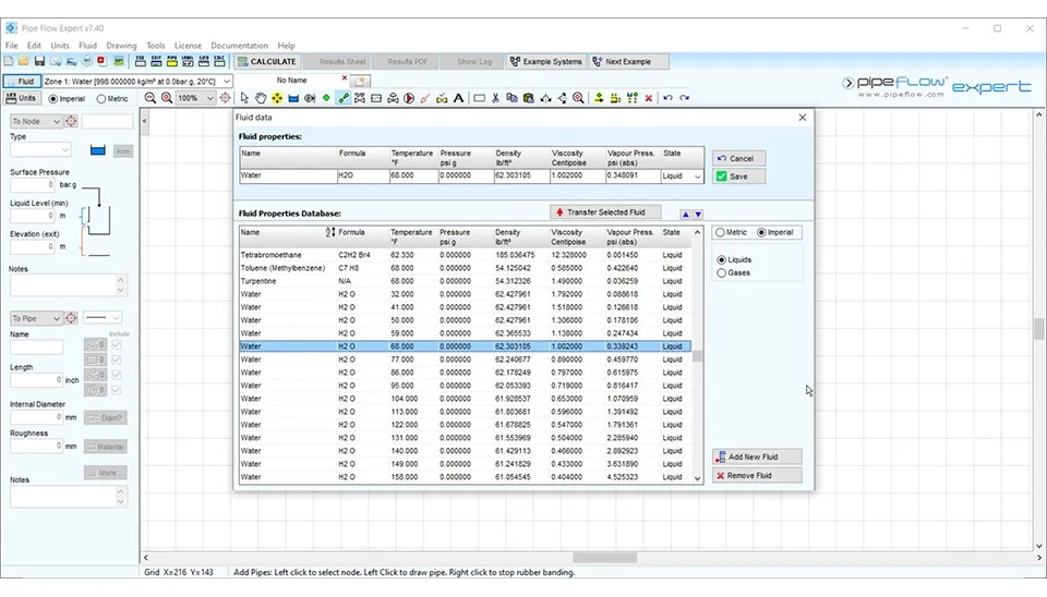
َAt first, by clicking on the fluid part and selecting the change fluid, you can access the fluid data window and select the desired fluid, either gas or liquid. Moreover, you can add the desired fluid if it is not in the list in Fig 2.
When setting up a water distribution network in Pipe Flow Expert, it is crucial to configure the correct unit settings to ensure the system's parameters are accurate and consistent. As shown in Fig. 3, the configuration window provides options to customize units for various system parameters, such as length, diameter, pressure, flow rate, temperature, and density. The Unit Settings tab allows users to switch between imperial and metric systems by selecting the corresponding option at the bottom of the window. This flexibility ensures that engineers and designers can work with their preferred unit system or adapt to the project's requirements.
In this example, because we are going to explain the design of a water distribution network, we selected the default option, which means water at 68 degrees Fahrenheit. The second important window is related to the unit part, which you can see in the following picture, Fig 3.
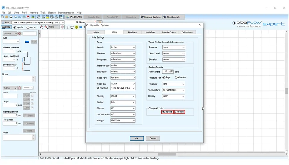
In this section, you can select one of these systems, Imperial or Metric. In this example, we select the imperial system.
For changing the fluid or selecting desired units, there are different ways, such as in Figs. 4-a, b.
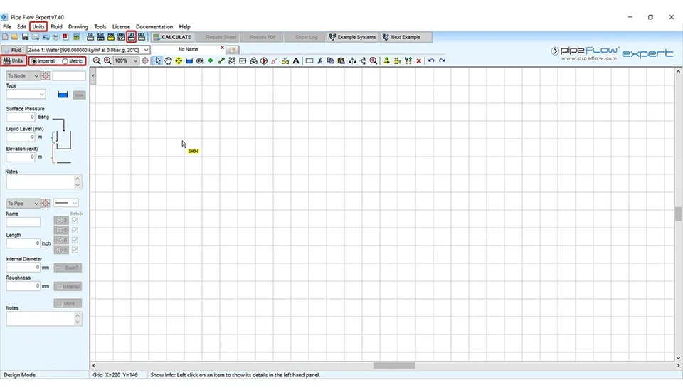
According to Figs. 4-a, b, you can have the same results by selecting each of these icons. For changing fluids, you can select the fluid menu from the menu bar. You can also click on the fluid data icon, which is shown in Fig. 4-a. For changing units for the water distribution network with pipe flow expert software, you have different ways, like selecting the unit menu from the menu bar. Also, you can select the icon related to units from the units and preferences section or select the unit icon. You can choose the imperial/metric part directly, as shown in Fig. 4-b.
Now, for designing a water distribution network by using the pipe flow expert, Fig. 5, just follow these five steps, including:
Step 1: Add tank
Step 2: Adding join point
Step 3: Add pipes
Step 4: Add fittings
Step 5: Add pump
Step 6: Add control valve (FCV, PRV and BPV)
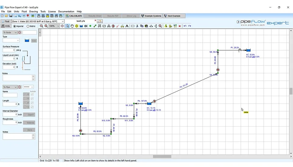
Fig. 5. An example for water distribution network using pipe flow expert software | An example of pipe flow expert software | Online training on water distribution network in pipe flow expert
To consider the main tank to start designing the water distribution network, activating this option is as simple as clicking on its icon that is shown in Fig. 6. After that, it is time to input data related to the main tank, such as surface pressure, liquid level and elevation (exit). These inputs are critical for ensuring the accuracy of the simulation and achieving a well-balanced design. Properly defining the surface pressure helps in simulating realistic conditions, while the liquid level and elevation data ensure optimal flow and pressure distribution throughout the network. By carefully entering these values, users can avoid potential errors in the system and ensure that the main tank operates as intended within the overall network configuration.
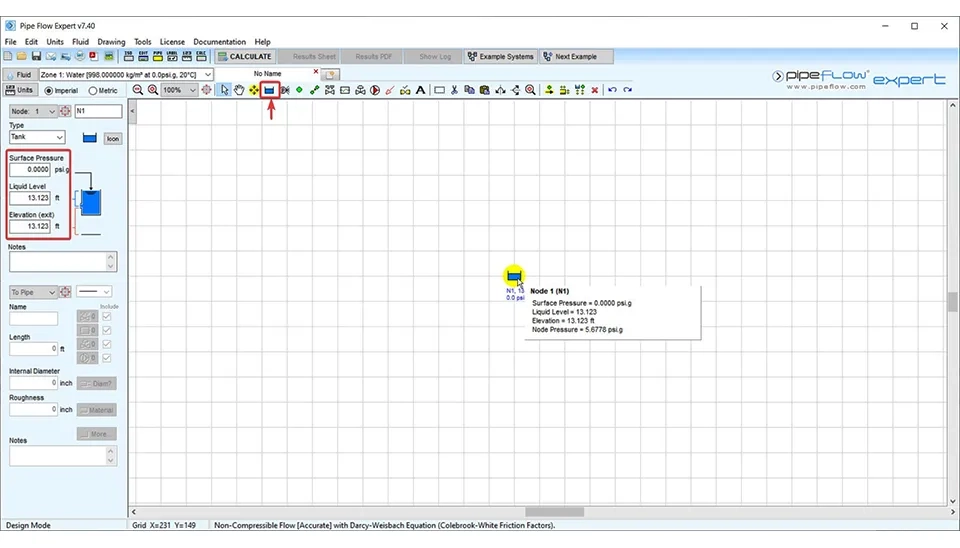
When there is a water distribution network and the tank level is open to the atmosphere, the surface pressure is set to zero. The liquid level in this example is considered 13.123 ft; you can input your desired value. Elevation is the distance between the tank bottom and the Earth surface. In this example, it is considered 13.123 ft.
After defining the tank, now it is time to add a node. A node needs to input the special data. The information that is used for the nodes is elevation of join (Fig. 7). Moreover, there are demands in and demands out, and you can edit them by clicking on the “Edit” icon. In set flow demands, you can choose the units for demands in and demand out.
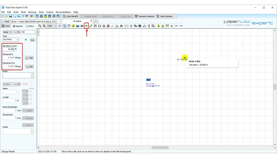
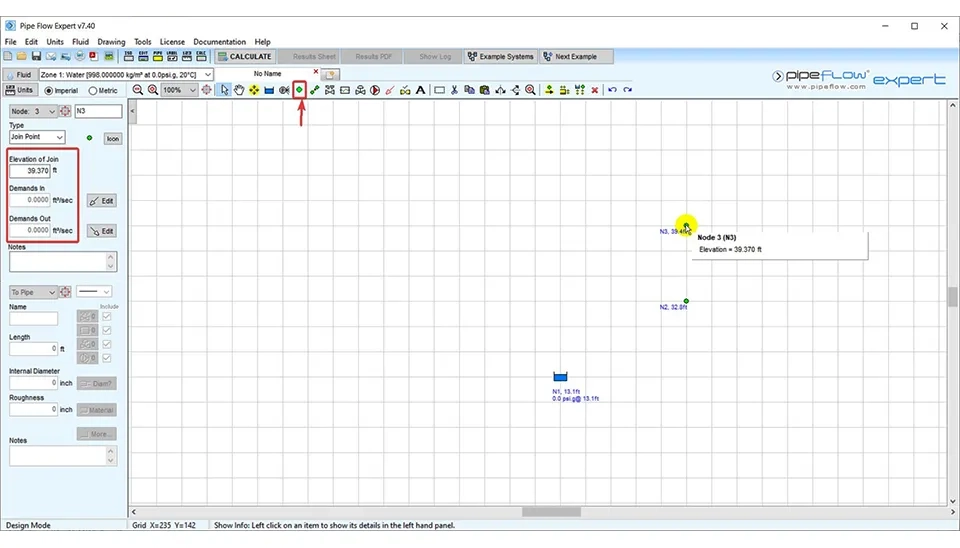
In this example, the elevation of the join is considered 32.808. You can definitely put your intended value according to your project. Sometimes in a water distribution network, there can be demands in a node or demands out of a node, Therefore,we can use demands in/out from this section. In the following, the next node is defined in the same way. The elevation of this joint point is considered 390.370 ft (Fig. 8).
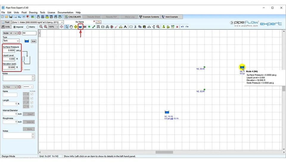
Furthermore, the first destination tank in this water distribution network is defined. The surface pressure for this tank is zero. It is assumed that the liquid level in this tank is zero and there is no water in the destination tank. The elevation of the tank in question is 32.808 ft (Fig. 9).
In this step, it is time to add pipes. For this purpose, click on the relevant icon as shown in Fig 10. The default pipe configurations are displayed in the pop-up window. In this window, the pipe properties are as follows: Stainless steel pipe is being considered. The length of the pipe is considered to be 10 feet, the diameter of the pipe is considered to be 4.026 inches and the roughness of the pipe is considered to be 0.002 inches as default.
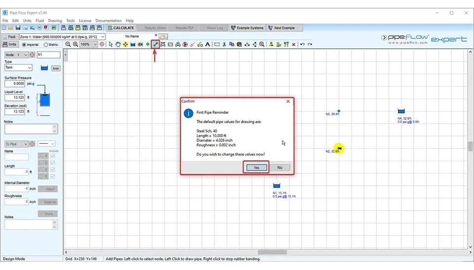
If you want to change the material of the pipe and these values of length of the pipes, the diameter of the pipes, and the roughness of the pipes , simply click on "Yes." After that, you will have access to pipe data. In this window (Fig. 11), click on the material option.
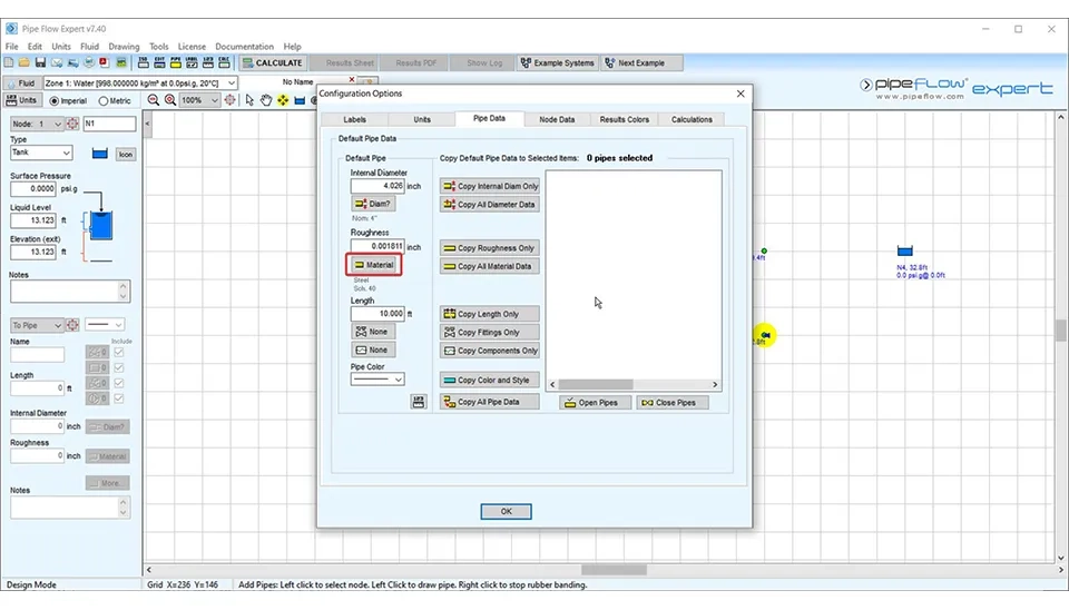
By clicking on the material option, the window related to different materials is displayed (Fig. 12). In this list, you can select the intended material for the pipe. As well as adding the new material if it is necessary.
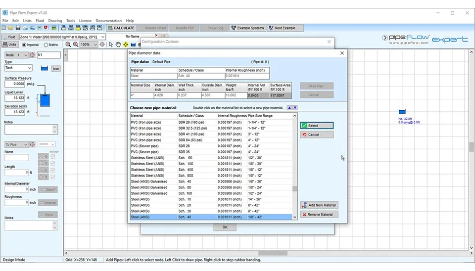
In this example, considering that HDPE (High-Density Polyethylene) is an appropriate material for the pipes of water distribution networks, HDPE pipe is selected (Fig. 13).
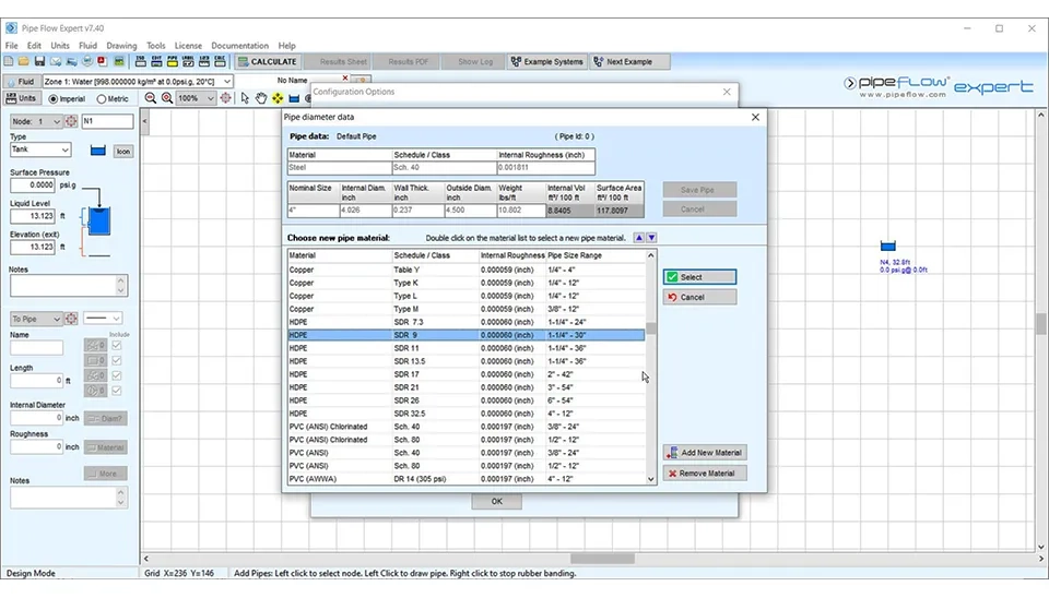
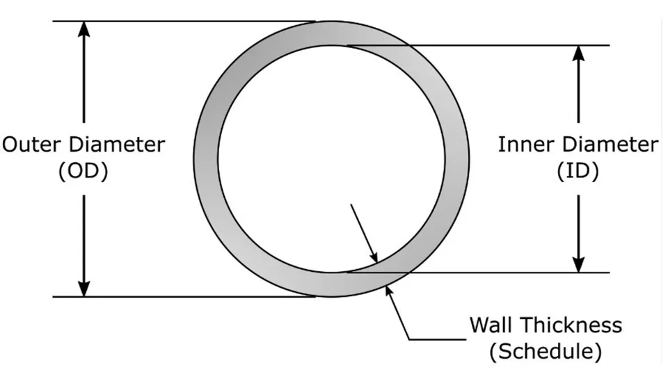
The HDPE pipes have different values for SDR. The SDR, or standard ratio in pipe, is the ratio. It means the ratio of nominal outer diameter to nominal wall thickness. You can see the outer diameter (OD), the inner diameter (ID) and the wall thickness in (Fig. 14).
In this example, the HDPE pipe with SDR 9 is selected. After selecting that, the nominal size is selected as shown in Fig. 15.
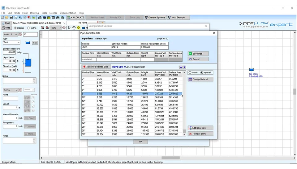
By selecting the nominal size, the selected size is transferred up the window (Fig. 16). This feature simplifies the process of choosing the appropriate pipe dimensions by automatically transferring the selected parameters to the main configuration panel. The user can then verify or adjust the values directly in the main window, ensuring accuracy and efficiency during system setup. Additionally, the ‘Save Pipe’ button allows users to finalize their selection and store the data for further calculations, streamlining the design process.
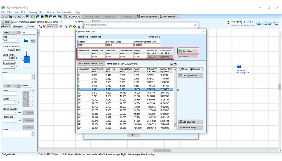
According to Fig. 16, in this example, the nominal size is considered 8 inches. Therefore, the other pipe properties are set automatically. These pipe properties include the internal diameter (in inch), the wall thickness (in inch), the outside diameter (in inch) and the weight (in lbs/ft). In this step, the values of the internal volume (in ft3/100 ft) and the surface area (in ft2/100 ft) are calculated by the pipe flow expert software. Now you can select the save pipe option in order to save the changes.
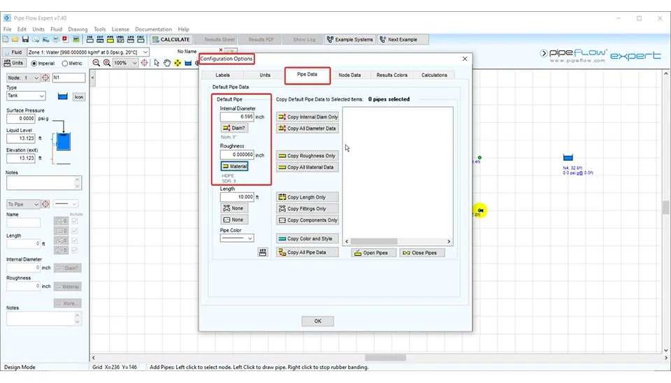
You can see the default pipe that you set in fig. 17, including the internal diameter of 6.595 inches and the roughness of HDPE SDR 9 pipe of 0.0006 inches. click on “OK” to save this data. Moreover, in the pipe data tab, you can use “copy internal diameter only” if you want to apply changes to a pipe or select "copy all diameter data” for applying to all pipes. You can do the same for roughness, fittings or length of the pipes. In this tab, the section pipe color can be very helpful in complex hydraulic systems.
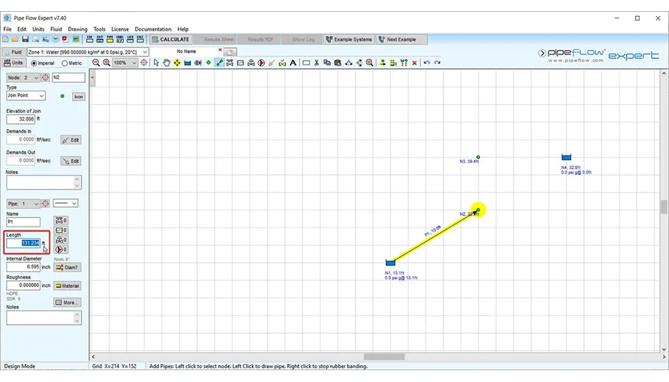
Another property of the pipe is length. One simple way to input the pipe length value is by using the section displayed in Fig. 18. In this example, the length of the pipe is considered 131.234 ft. Since the default pipe material has changed, inputting the length of the pipes needs to be done. Fig 19-a.
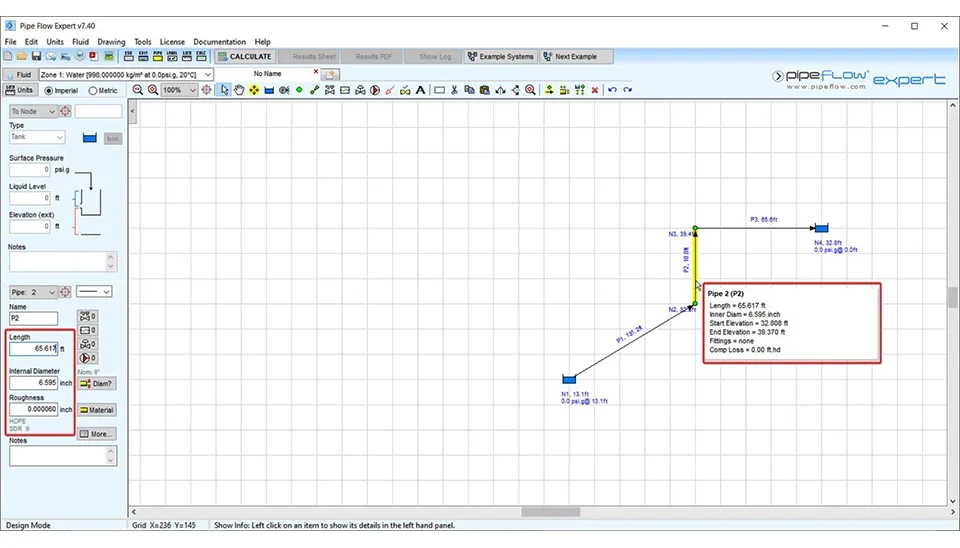
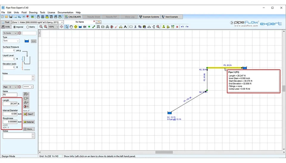
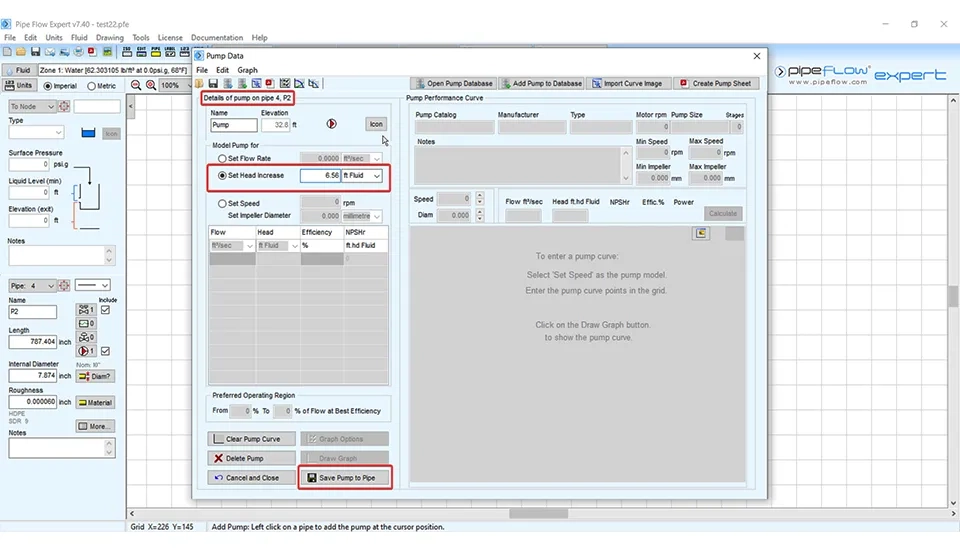
For pipe number 2, the length is considered 65.617 ft; see Fig. 19-b. Repeating the process for the next pipe. Therefore, pipe number 3 is considered 26.247 feet. Note that when you hold the mouthpointer over different sections, you can see more information about the desired part (hydraulic components). For example, in Fig. 19-b, you can see the number of the pipe and the name of the pipe. Moreover, you can see other information, like: The length of the pipe is considered 65.617 ft, the inner diameter is 7.874 inch, the start elevation is 32.808 ft, the end of elevation is 39.370 ft, and the entry fittings K value is not considered in this part of water distribution of network Pipe 4 (P2), the exit fittings K value is 0.84, and the comp loss in pipe flow expert software indicates that the software calculates the pressure drop caused by various components of the water distribution network (such as fittings, valves, etc.) in units of feet of head. In P2 the comp loss is zero and “the pump @ fixed head” is related to the pump operating at a constant head. For this pipe, the pump @ fixed head is 6.56 ft. hd.
When you select the pipe and click to join the nodes, this command remains active; if you want to inactivate it, use “Esc” on the keyboard or just right-click with your mouth or click on show item information .
In a water distribution network, using a variety of fittings is necessary for many reasons. For example, change of flow direction and size of pipes, connecting pipes and preventing leakage in distribution networks. To perform this action in the pipe flow expert software, click the corresponding icon as shown in Fig. 20.
When you click on this icon, you can access pipe fitting friction coefficients. Look at all the different fittings that you can select based on the water distribution network you are thinking of (Fig. 21). The pipe fitting friction coefficients window provides an extensive list of fittings that can be added to a specific pipe segment within the water distribution network. Each fitting in the list is accompanied by its friction coefficient, which contributes to the overall pressure loss in the system. By selecting a fitting, such as bends, valves, or reducers, users can view its details, including size, description, and associated friction value. These values are critical for accurately modeling the hydraulic behavior of the system and ensuring efficient water flow.
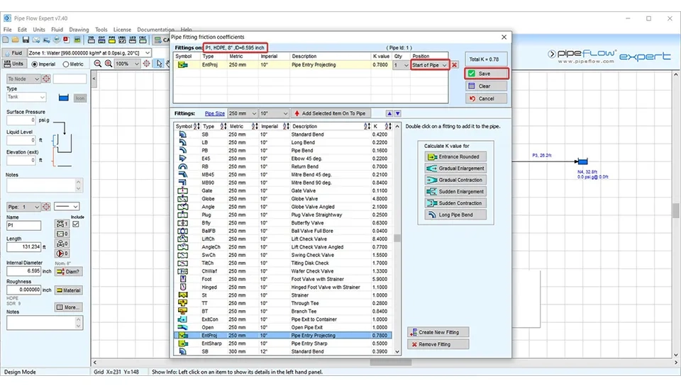
According to Fig. 21, the fitting on pipe 1 is considered EntProj type (pipe entry projecting) with 10 inches for this example. When selecting the desired fitting, the selecting fitting is displayed on top of the window. The K value for this choice has been 0.78. You can also select the position of the fittings on the pipe, meaning you can specify whether the fitting is located at the start of the pipe or the end of the pipe and then save it. These descriptions are about pipe 1. You can also do the same thing with other pipes.
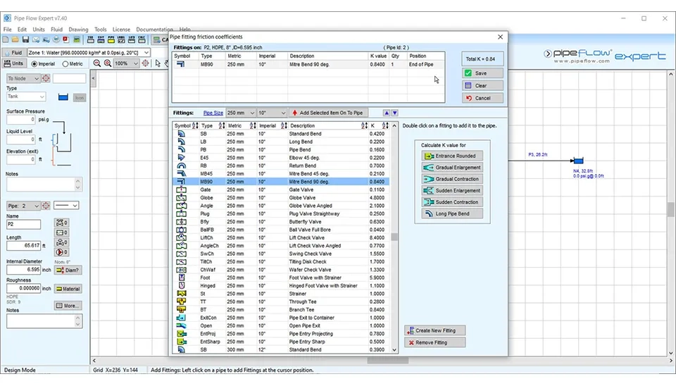
According to Fig. 22, for pipe number 2, you can use the MB45 type of fittings (10 inches for this example). The K value for this selection is 0.84 and the position of this fitting is at the end of the pipe.
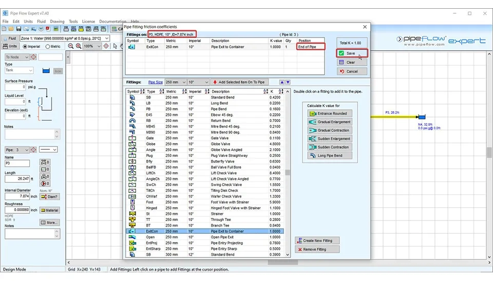
And the last fitting on the right of the water distribution network in question in this example, meaning on the pipe 3 is ExitCon (pipe exit to container) fitting at the end of the pipe. The K value for this fitting is 1. When there is a tank and a pipe is connecting with the tank, this type of fitting is used (Fig. 23).
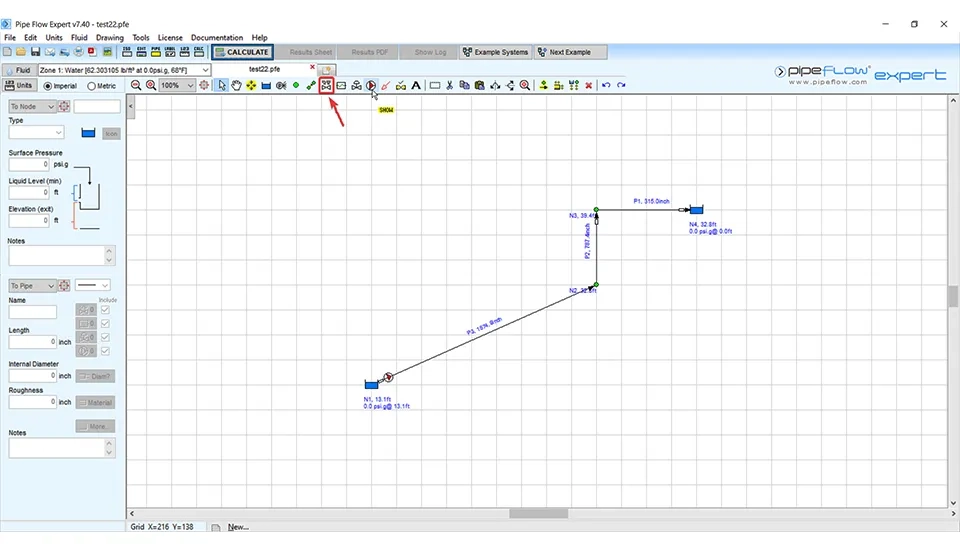
If you go back and check the elevation of nodes again and focus on their values, you need to realize that the main tank is located at the lower elevation compared to the following point, and the same applies to the next node. In this situation, the water is not conveyed by gravity and a pump, which can be used to supply water to the nodes, ensures an adequate water pressure in the water distribution network. Select the pump icon as shown in Fig. 24.
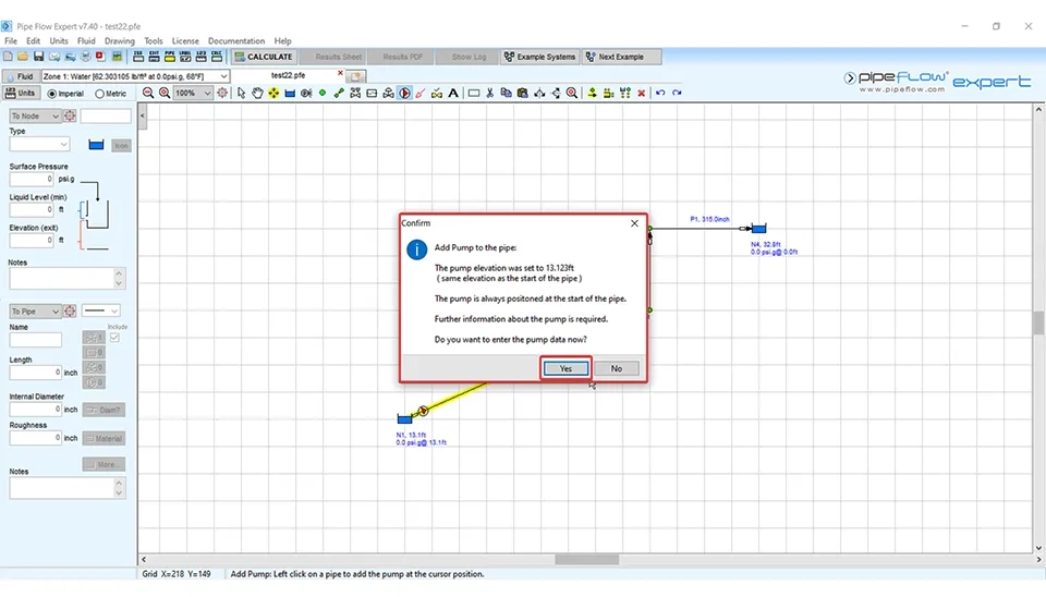
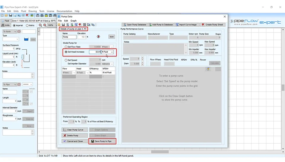
After clicking on the pump icon, a window is displayed that is about the pump elevation. The pump pointed at the start of the pipe. It is possible to click on the “Yes” option to enter the pump data in Fig. 25.
The pump data is shown in Fig. 26. In the “model pump for” section, the desired pump can be considered in three ways. The first way is based on flow rate, the second is based on head increase (used in this example) and the last way is based on speed and set impeller diameter. If you select the last way, it is possible to access the pump database and select the desired pump from the pump library (Fig. 26). In the pump library, you can access various data about pumps and search different pumps, checking the pump features and selecting the best choice based on your desired water distribution network.
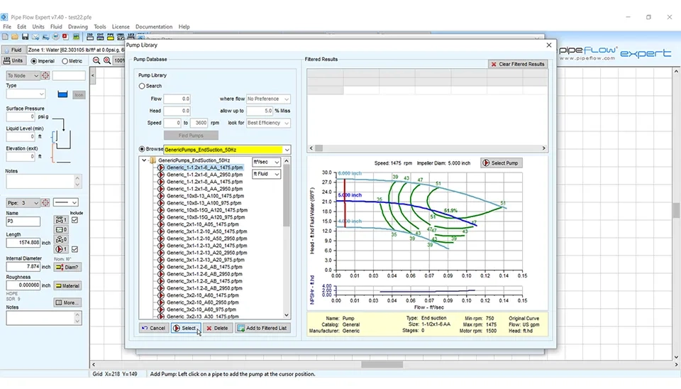
By using this part, you can find the suitable pumps based on your needs.
Search based on Flow: You can search for the suitable pump based on the various flows. The pumps that work in the specific flows are identified and selected the best of them.
Search based on head: You can search the pump based on head. This option allows you to find the pumps with the desired head.
Search based on speed: In this section, you can select pumps based on pump impeller speed. This option is very important in selecting the best pumps in terms of efficiency.
These results are displayed in filtered results.
In the pump library, there is a part called browse. In this part, there is a list of pumps. You can select one of them and analyse the pump performance charts in the right of the pump library window.
Q-H curve: This curve demonstrates the relationship between flow rate and the head. You can have sufficient information about the pump’s performance in different conditions.
Isobar lines: The isobar lines indicate the head pump at different flow rates and pump efficiency.
NSPH charts: These charts represented the minimum acceptable suction pressure to prevent the cavitation phenomenon in pumps.
After selecting the desired pump, you can save the pump to the pipe.
In this water distribution network, because the node after the tank is at a lower elevation compared to the next node, we need to use a pump on the pipe connecting these nodes (Fig. 27-a, b).
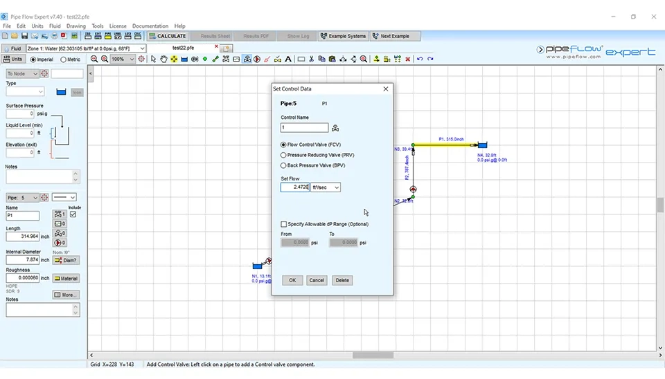
The control valves are used to regulate and control the flow in the water distribution network. These valves have different types, such as FCV (Flow Control Valve), PRV (Pressure Reducing Valve) and BPV (Back Pressure Valve) (Fig. 28).
In this example, for controlling the flow rate, the FCV type of the control valves on P3 pipe (Fig. 29) is used. The Flow Control Valve (FCV) ensures that the desired flow rate is maintained in the system by automatically adjusting the pressure and flow dynamics in the P3 pipe. This setup is particularly useful in complex systems where precise flow management is required to optimize performance and prevent issues such as overpressure or flow imbalance. As shown in Fig. 29, users can easily set the required flow rate value and specify allowable pressure ranges to ensure operational stability and efficiency. The intuitive interface simplifies configuration, making it accessible for both novice and experienced users, while providing flexibility to adapt the valve settings to a wide range of applications.
In this part, if you want to use pressure-reducing valves (PRV) or back pressure valves (BPV), select them. This process involves placing and configuring the appropriate valves and pipe segments to control pressure and ensure optimal flow.
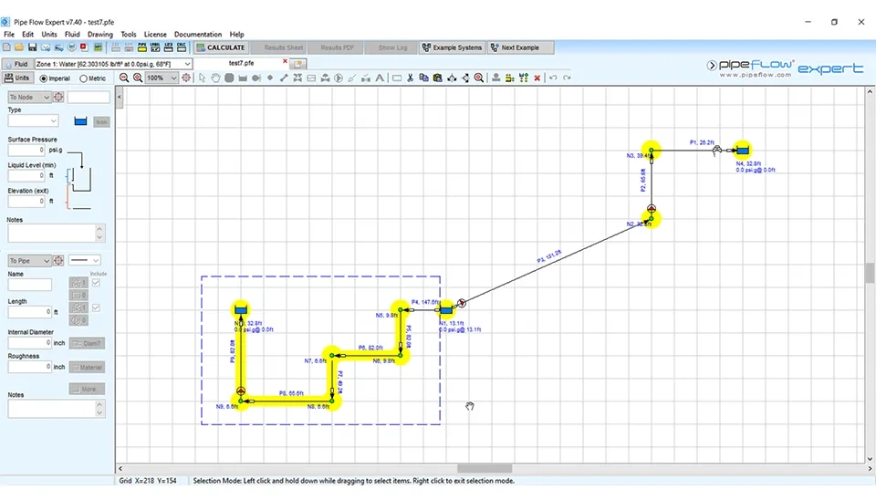
Using the detailed steps outlined earlier, users can replicate the methodology for consistent and accurate results. The flexibility of the software allows for the easy addition and adjustment of components to meet specific design requirements.For designing the left section of the water distribution network (fig. 30), using pipe flow expert software, you can do the same steps that were mentioned before, according to tables 1 and 2.
Flow Expert Software
In table 1, there is the name of each pipe, the length of pipes in feet, and the internal diameter of pipes in inches. In table 2, there is the name of nodes from number 5 to 9 and their elevation of join and the elevation (exit) in ft related to Node number 10. You can use this information as input data for designing the left part of the water distribution network with pipe flow expert software.
Table. 1. Summary of Pipe Information | Advanced Training on Water Distribution Network in Pipe eFlow Expert
Name | Length (ft) | Internal Diameter (inch) |
P4 | 147.638 | 3.937 |
P5 | 82.021 | 7.874 |
P6 | 82.021 | 7.874 |
P7 | 49.213 | 7.874 |
P8 | 65.617 | 7.874 |
P9 | 82.021 | 3.937 |
Table. 2. the elevation of nodes| Online Training on Water Distribution Network in Pipe Flow Expert
Name | Elevation of Join |
N5 | 9.843 |
N6 | 9.843 |
N7 | 6.562 |
N8 | 6.562 |
N9 | 6.562 |
Name | Elevation (exit)(ft) |
N10 | 32.80 |
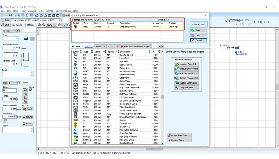
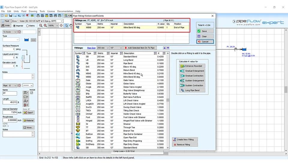
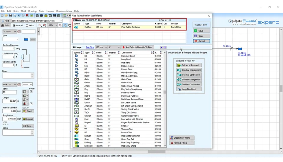
In the following, you can see the data for fittings used in this section of the water distribution network, Fig. 31 a-f. These figures provide a detailed breakdown of the types and specifications of fittings incorporated into the network. The fittings data includes critical parameters, such as dimensions, material types, and associated loss coefficients, which are essential for accurate modeling and performance analysis. The visual representation in Fig. 31 a-f further helps in understanding the placement and role of each fitting within the system.
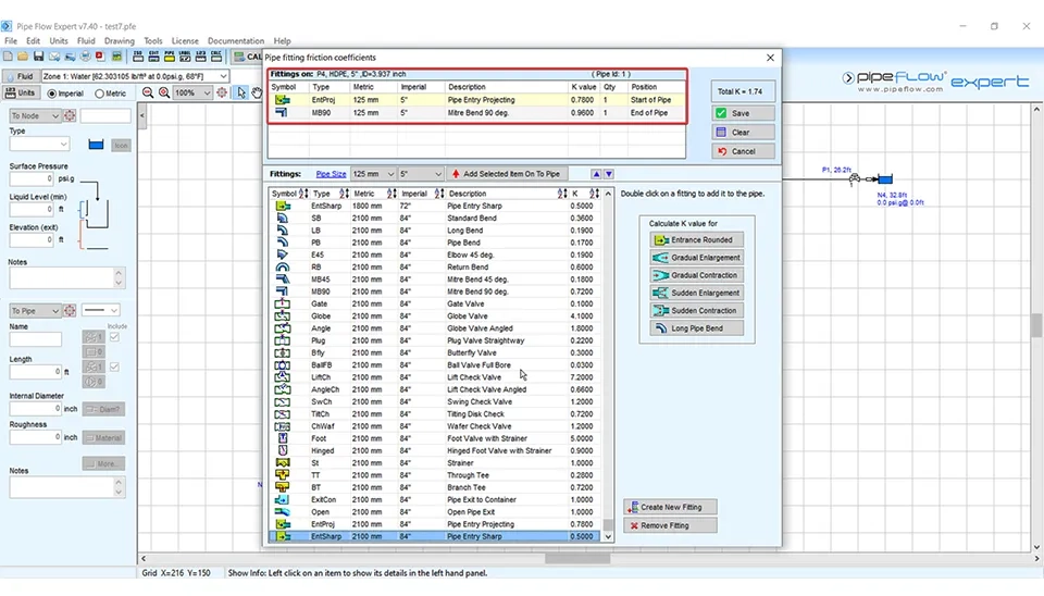

According to these figures, for P4 pipe, we use two types of fittings. The first is the EntProj type at the start of the pipe and the second is the MB90 at the end of the pipe. You can see other properties in Fig. 31-a.
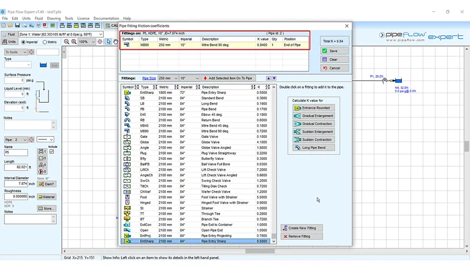
About the P5 pipe, we use just the MB90 type of fitting at the end of the pipe. In figure 31-b, you can see the details.
In pipes P6, P7 and P8, the fitting used is the MB90 at the end of the pipe.
In pipe P9, the fitting type is ExitCon at the end of pipe Fig. 31-f.
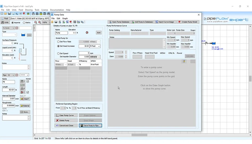
In addition, in pipe P9, we need to use the pump to supply water to the destination tank at an elevation of 32.808 ft. You can see pump data related to this pipe in Fig. 32.
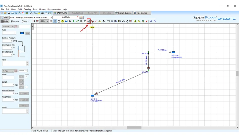
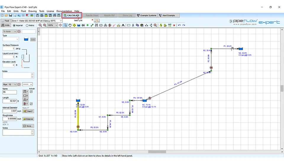
After adding nodes, the tank, the pump and all the fittings, it is time to calculate the result of the system by clicking on its icon (Fig. 33). The calculation process evaluates the entire water distribution network, identifying flow rates, pressures, and potential inefficiencies. This step ensures that the system operates optimally, meeting the design requirements for performance and reliability. By using the 'Calculate' button, users can quickly obtain detailed results and make any necessary adjustments to improve the system's overall efficiency.
The pipe flow expert presents the results log. This software gives us a lot of detailed information about the system that is designed.or example, the calculation engine, start calculations, final solution details and configuration. When checking the network, if there is a problem, it is displayed and you can re-design the system, but if this message “No issues to report" is displayed, it means that the model has been solved well, and you can also see this sentence that the solution values are displayed on the drawing (Fig. 34).
If there are any problems, all of them are displayed as comments and warnings in this section, and you can resolve and re-design the water distribution network again by making the necessary changes. For example, if the velocity in pipes is not in virtual range by changing the pipe diameter, it will be corrected.
According to the continuity equation, the velocity in the pipe is obtained from the following equation (Eq. 1):
Q=AV;A=d24 v=QA=Qd24 (1)
In this equation, the velocity in the pipe is displayed with v, Q is the flow rate in the pipe and d is the pipe diameter. It is emphasized that, if the velocity in the pipe is high in the pipe, based on this equation, by increasing the diameter of the pipe and, as a result by increasing the pipe cross-sectional area, the velocity in the pipe is decreasing. You can do the same for other hydraulic situations in the water distribution networks.
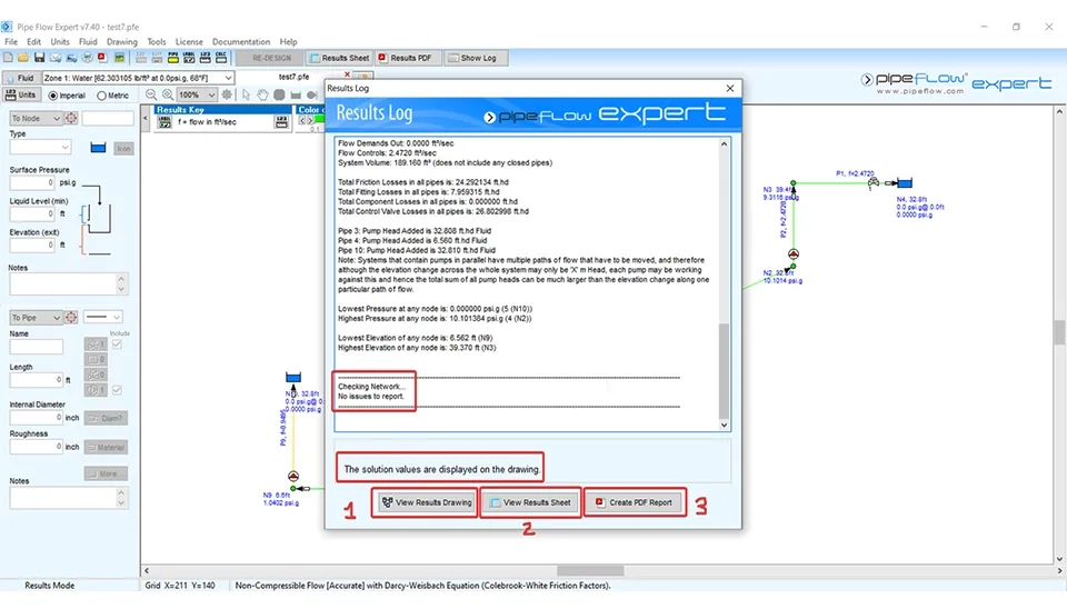
According to Fig. 34, the pipe flow expert presents results in three modes.
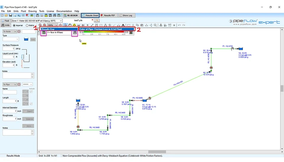
1. View results drawing Fig. 35: In this part, you can see the results in a spectrum of colors. By clicking on “Labels” in the result key, you access the label tab in configuration options and check all of the options that you want to show on the result drawing sheet. By clicking on the “123” icon, the tab units in configuration options are displayed. You can make the changes if you need. By clicking on “color” in box number 2 in Fig. 35, you can see the results color tab in configuration options and apply the changes.
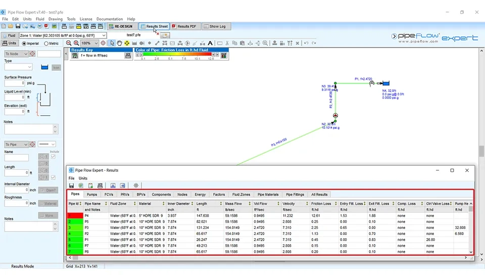
2. View results sheets: You can see more details in this section (number 2 in Fig. 35). You can also see the different tabs in this sheet (pipe flow expert results) in Fig. 36.
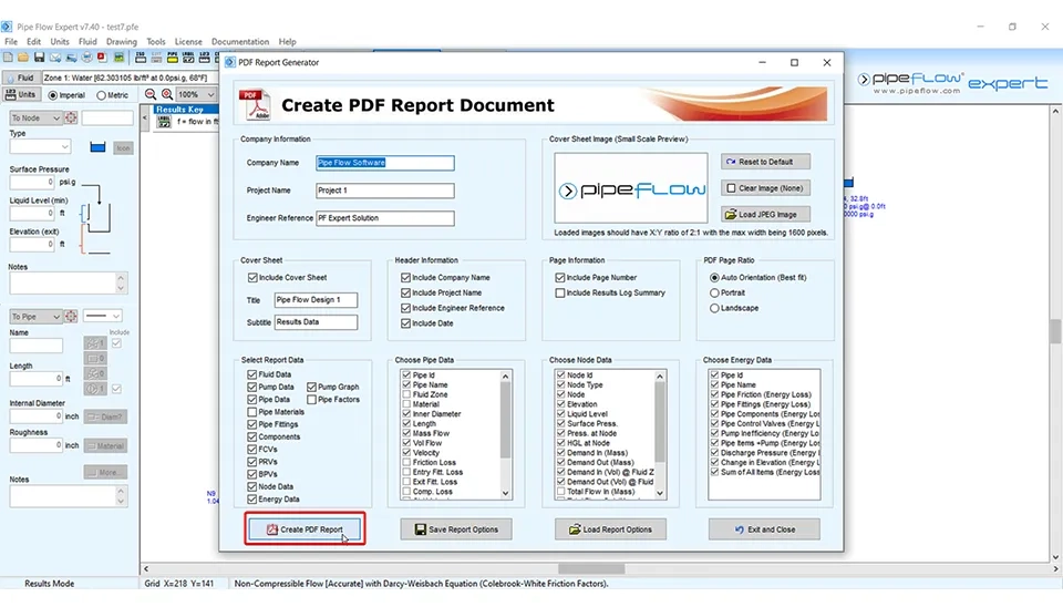
3. Create a pdf report: An interesting result in the pipe flow expert software is this part. This software represents a fully pdf report that you can see all of the details about your design of the water distribution network in Fig. 37.
Click here to download the complete PDF report of the water distribution network design
Move : If you want to move components, you just need to click on the related icon from the drawing tool buttons.
Delete: If you want to delete a component in a water distribution network, first select the desired component and then click on the delete icon. If you also want to delete a section part of a water distribution network, by selecting its icon and the delete icon, you can eliminate it.
Cut, Copy, Paste : Cut, copy and paste in the pipe flow expert have the same application in other software.
Pan : Pan is used for moving in different parts of your hydraulic model. Click on the related icon from the drawing tool buttons.
Since the water distribution network often consists of many pipes, tanks, fittings and hydraulic components, using powerful software for the design and analysis of the system is very necessary. A water distribution network is a complex system that requires precise calculations and careful planning to ensure efficient functionality. Accurate design and analysis of such systems play a crucial role in managing water resources effectively, minimizing energy consumption, and maintaining consistent water pressure throughout the network. The pipe flow expert is useful software in a water distribution network. In this article we brought up an example and we carried forward the software training with this example step by step. Finally, the pipe flow expert software created pdf results. In this detailed and insightful PDF report, you can see full information about your designing the water distribution network. The fluid data, pipe data, fittings, components, flow control valves (FCV), pressure-reducing valves (PRV), back pressure valves (BPV), node data and energy data are presented in tables in the pdf results. These detailed outputs enable users to review their designs thoroughly, identify potential issues, and make informed decisions for optimization. By leveraging the capabilities of Pipe Flow Expert software, users can significantly enhance their understanding and management of water distribution networks, making it an indispensable tool for professionals in water resource engineering and management.
Quick answers to common questions.
Keep reading


Comments
No comments yet
Be the first to comment
Share your thoughts and start the conversation.