In the past, engineers used manual methods and complex calculations to design and analyze wastewater systems. With the advancement of computer technology, various software programs were developed to simplify these processes. Unlike a water supply system, a sewerage system’s installation is much more costly and requires frequent maintenance, contributing to high operational costs. Research is ongoing to create cost-effective sewerage systems, with SewerGEMS V8i software being a key tool for designing optimal layouts and pipe diameters (Rajpurohit and Raol, 2016).
An efficient, sustainable, and economical sewer system is essential for engineers when planning and constructing one. This system transports wastewater or stormwater underground through manholes and conduits. Designing a sewer system requires modeling studies, which can be physical or numerical using software like InfoWorks and SewerGEMS. The project will create a GIS-based numerical model and conduct simulations with QGIS and Bentley SewerGEMS software (Kulkarni et al., 2021).
Bentley has introduced software called SewerGEMS as a solution to all the above problems to design a cost-effective and highly efficient sewer system in a short time. SewerGEMS software is one of the most advantageous tools for designing an economical and cost-effective sewer system that gives the best possible cost and layout of a large system which can have various pipe diameters, by considering the flow velocity in the pipes (Chaudhary et al., 2020).
Fig. 1. Typical sanitary sewer network diagram used for hydraulic simulation and modeling in SewerGEMS software.
1. The SewerGEMS Software Overview and Modeling Capabilities
Numerous up-to-date numerical models are available for conducting stormwater system flow loading. One widely used software program is SewerGEMS, which is tailored explicitly for analyzing and designing sewage systems. It offers built-in hydraulic tools and provides a streamlined environment for experts to analyze, plan, design, and operate sewer systems (A.Kulkarn et al., 2021).
SewerGEMS software is a powerful tool for analyzing, designing, and operating sanitary and combined sewer systems. It offers a comprehensive suite of features for modeling and simulating the hydraulic behavior of wastewater systems.
It is also a user-friendly software compatible with ArcGIS and AutoCAD tools. SewerGEMS offers many unique benefits, including:
Time and effort savings: The program allows hydraulic analyses to be conducted quickly and accurately, reducing the need for redesigns and a complete restarting from scratch.
Accuracy in analyses: SewerGEMS allows users to analyze data accurately and reliably, aiding in crucial system design and maintenance decisions.
Integration with GIS: Engineers can use available geographical data in the GIS system for system analysis and design, enhancing the accuracy of results and work efficiency.
Ease of Use: The program features a simple and user-friendly interface suitable for sewage and stormwater engineers at various expertise levels.
Fig. 2. SewerGEMS training example: Detailed profile view used for wastewater system design and depth analysis.
2. Wastewater System Design Using SewerGEMS Software
The design of the sewage system includes numerous major steps. SewerGEMS assists water and sewage engineers with designing, modeling, and analyzing the system.
The main steps include:
1. Gather the initial information: determine the flow rate, and analyze the geology and topography desired.
2. Modeling sewage systems:
importing the geography map of the desired area, and adding components such as conduits, manholes, lift stations, pumps, and wet wells.
3. Define component specifications: determine the diameter, velocity, and length of the pipes, and specify pumps and pumping station specifications.
4. Hydraulic analysis : import the flow rate and run the model to examine the flow, velocity, and pressure in the sewage system.
5. Optimization and evaluation: the analysis of the results and identification of the weaknesses and the need for optimization, as well as providing solutions to prevent overflow and disruption.
6. Reporting: present the modeling results, drawing and appropriate suggestions for preventing errors in the model, as well as calculating the costs related to the construction and maintenance of the sewage system.
2.1. Relation Between Water Supply and Wastewater Flow in SewerGEMS Design
Municipal wastewater is derived largely from the water supply. However, a considerable portion of the water supply does not reach the sewers. This includes water used for street washing, lawn sprinkling, firefighting, and leakages from water mains and service pipes. Products and manufacturing processes may also consume a small portion of water. Also, many homes and other establishments that are not served by a sewerage system may use the city water supply but utilize on-site wastewater treatment and disposal.
On the other hand, infiltration/inflow and water used by industries and residences obtained from privately owned sources may make the quantity of wastewater greater than the public water supply. In general, the average wastewater flow may vary from 60 to 130 percent of the water consumed in the community. Many designers frequently assume that the average rate of wastewater flow, including a moderate allowance for infiltration/inflow, equals the average rate of water consumption. Average wastewater flows from residential, commercial, industrial, institutional, and other sources may be obtained from careful consideration of local water consumption data or by using wastewater generation rates published in the literature (Syed R. Qasim, Second Edition).
The purpose of a wastewater collection system is to collect and convey the wastewater from a community's homes and industries. The water carries the wastes as either dissolved or suspended solids. The wastewater in collection systems is usually conveyed by gravity, utilizing the land's natural slope. Wastewater pumps are used when the slope of the land requires lifting the wastewater to a higher elevation for a return to gravity flow. Pumps and other mechanical equipment require extensive maintenance and costly energy, so their use should be avoided whenever possible. Thus, the location and design of a collection system's components are strongly influenced by its service area's topography (surface contours).
2.2. Essential Requirements for Hydraulic Design in SewerGEMS
Municipal wastewater mainly originates from the water supply, but not all of this water reaches the sewer system. Some are used for street washing, lawn sprinkling, firefighting, and leaks, while others may be consumed by products and manufacturing processes. Additionally, homes and businesses not served by sewers often use city water for on-site wastewater treatment.
Inflow and infiltration (I/I), along with water from privately owned sources, can increase wastewater volumes to the levels beyond the public water supply. Average wastewater flow typically ranges from 60% to 130% of community water consumption. Designers usually assume that this flow rate matches water usage.
2.2.1. Calculation of Wastewater Generated by Urban Systems in SewerGEMS
Ideally, a wastewater collection system should be designed to convey the estimated peak flow from its service area when the area has reached its maximum population and has been fully developed commercially and industrially.
However, under these circumstances, the sewers are designed to convey peak flows estimated to occur within an appropriate design period, ranging from 10 to 30 years.
Therefore, once the design period has been determined, design flows that will occur during the period are calculated based on the estimated population, per capita wastewater discharge, and industrial and commercial wastewater discharges at the end of the period.
Henrietta City was selected to design wastewater systems. The city’s per capita flow from residential sources is about 92.5 gallons per capita per day (gpcd).
According to the predicted population in 2054, the demand was calculated at 29.32 gal/s household flow. About 80% of this flow is converted into wastewater because about 20% of the demand leaks into the earth throughout the pipes’ breaks (Ryuichi et al . 2019). estimated that exfiltration in a leaky sewer in Berlin ranged from 2.3% to 18.8% (Rieckemann et al . 2006). reported that the exfiltration ratio in Rumlang, Switzerland, ranged between zero and 15% (Rieckemannet al . 2005), and Ellis et al. estimated exfiltration rates of 5–10% in artificial leaky sewers (Ellis et al., 2003).
To estimate demand for 2054, the population in 2054 must be predicted; therefore, to familiarize yourself with ways to assess demand for Henrietta City, please read the WaterGEMS Training article (parts 2.1.1 and 2.1.2).
Accordingly, the main sewage flows for designing wastewater include residential, industrial, rainfall-induced runoff, and infiltration.
2.2.2. Determining The Amount of Household Wastewater Minimum and Maximum
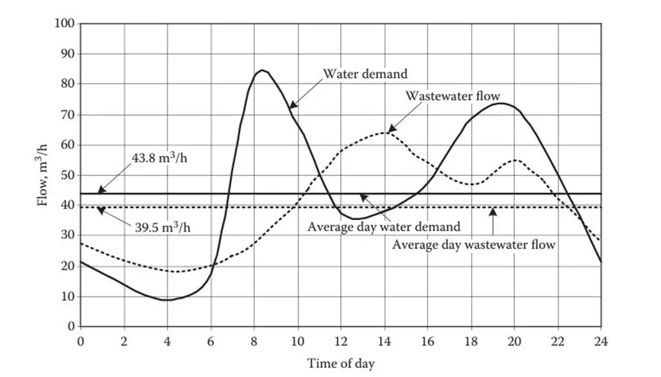
Like water demand, wastewater flows also vary in terms of time of the day, day of the week, weather conditions, and year's season. Under dry weather conditions, the daily wastewater flows show a diurnal pattern exhibiting a peak and a minimum in 24 hours. The diurnal wastewater flow parallels that of water demand with a time lag of a few hours (Fig. 3).
Fig. 3. Output data table (FlexTable) in SewerGEMS displaying key attributes like diameter and length for sewer network modeling.
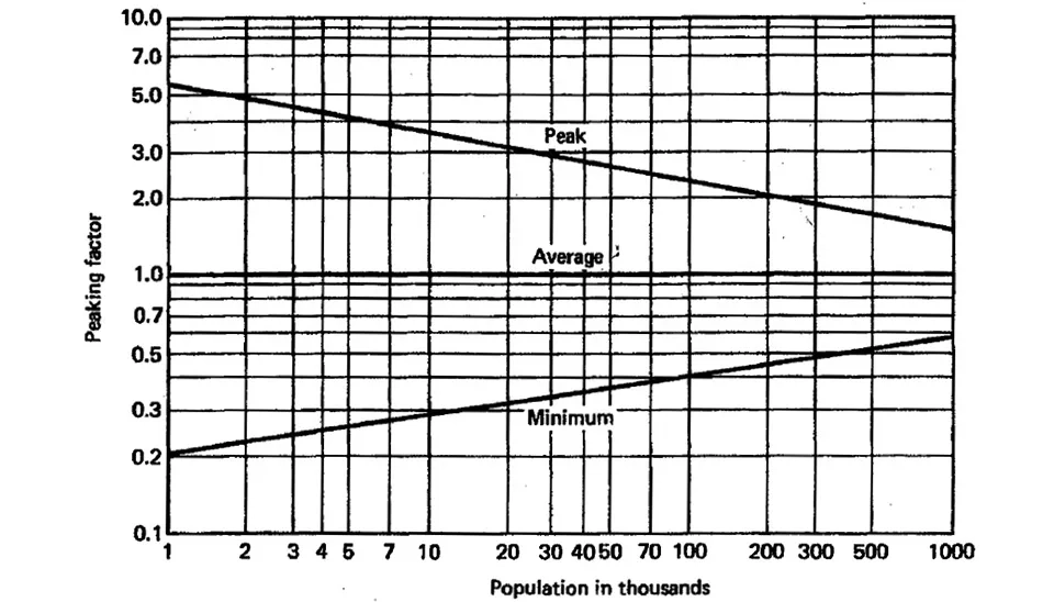
We generally estimate the hourly peak and minimum dry weather flows using several equations and graphical relationships developed from case studies. The ratio of hourly peak to the daily average and hourly minimum daily average flows depend upon the contributing population (Syed R. Qasim, Second Edition & Tchobanoglous and Shroeder, 1985).
In this way, minimum and maximum flow are calculated based on total wastewater flow. The maximum flow rate is used for designing, and the minimum flow controls flow conditions in the wastewater system. Minimum and maximum flow ratesare critical parameters in wastewater system design. They influence the size of pipes, pumps, and treatment plant components.
Minimum Flow Rate
The minimum flow rate in a sewer system refers to the lowest expected flow of wastewater. This low flow can cause several issues, including sediment buildup and clogging of pipes. Additionally, insufficient flow may reduce pumping station efficiency and negatively affect biological treatment process performance.
Factors Affecting Minimum Flow Rate:
1. Population Density: Areas with lower population density typically experience lower minimum flow rates.
2. Seasonal Variations: Water usage can vary significantly throughout the year in some regions, impacting the minimum flow.
3. Industrial and Commercial Activity: The activities of industries and commercial establishments can also influence the minimum flow rate in a sewer system.
Note: The minimum flow is used for designing when there is no information from sewage fluctuations in the wastewater system.
Maximum Flow Rate
The maximum flow rate refers to the highest flow levels that can be anticipated within a sewer system. It is crucial to monitor these rates because excessive flows can overwhelm treatment plants, resulting in poor effluent quality and potential overflows. High flow rates may lead to hydraulic overload and flooding within the sewer system (Muttil et al., 2022 & Syed R. Qasim, Second Edition).
Factors Affecting Maximum Flow Rate:
1. Peak Hourly Flow: This is the maximum flow rate that occurs during a specific hour, typically during peak usage times.
2. Rainfall Intensity and Duration: Heavy rainfall can significantly increase the flow rate, especially in combined sewer systems.
3. Infiltration and Inflow: The infiltration of groundwater and the inflow of stormwater can add to the overall flow, contributing to heightened flow rates.
Note: The maximum flow rate is used for areas where the maximum population is 1000 people.
Fig. 4. The Scenario Manager in SewerGEMS modeling, allowing engineers to compare different hydraulic design and operational states.
The minimum to average flows depend on the population. Larger cities have fewer deviations from the average than smaller cities. Many designers use the· "fixture-unit load" method for estimating peak wastewater flows for facilities such as hospitals, hotels, schools, apartment buildings, and office buildings (Syed R. Qasim, Second Edition).
Engineers should use caution with curves or parameters developed historically, since changing lifestyles (such as more women in the workforce instead of staying at home; water conservation; and increasing use of reclaimed water for residential irrigation) may result in attenuated peaks from residential flow (Paul Bizier, 2007).
Thus, the formula for wastewater minimum and maximum flow is as follows:
Formula maximum flow -—----> Mmax= 5/P0.167 ⇒ Kmax= 5/ 3.90.167= 3.98
The population in 2054 is the goal of this design; therefore, P is the population predicted in 2054, 3900 people. Thus, the population predicted for Henrietta city (World Population Review) is 3900. These formulas use population per thousand.
Apply peaking factors to each point (manhole) down through the system, thus generating the peak 1-hour flows for all sewer reaches in the system. The peak flows from Qavq1 are the Qmin values needed for self-cleaning design; those from Qavq2 are the Qmax values needed for capacity design (Paul Bizier, 2007).
2.2.3. Estimate Infiltration and Inflow (I/I) Into Wastewater System
Rainfall-runoff is divided into three parts: 1) A portion goes into stormwater systems; 2) A portion evaporates or is used by plants; and 3) the rest becomes groundwater. How much water seeps into the ground depends on surface type and soil, as well as precipitation patterns. Reduced permeability from buildings or pavements leads to more runoff and less groundwater. Groundwater flow can range from very low in dense areas to 25–30% of rainfall in sandy areas. Additionally, water from rivers can significantly influence the groundwater table, which changes over time.
Inflow includes rainwater and surface water entering a sewer system through connections like downspouts and sump pumps. Infiltration happens when groundwater seeps into sewer pipes, often due to ageing infrastructure. Rainfall affects the extent of inflow and infiltration (I/I), which reduces system capacity and can lead to sewer overflows, causing pollution (Pawlowski et al., 2013).
impact of High Groundwater
The presence of high groundwater levels results in leakage into the collection systems and an increase in the quantity of wastewater and the expense of its conveyance and treatment. This occurrence is of particular importance in the Northeast when spring snowmelt occurs. The amount of flow that can enter a collection system from groundwater infiltration may range from 0.01 to 1.0 m³/d·mm·km (100 to 10,000 gal/d·in.·mi) or more. The number of millimeter-kilometers (inch-miles) in a wastewater collection system is the sum of the products of sewer diameters, in millimeters (inches), times the lengths, in kilometers (miles), of sewers of corresponding diameters.
Estimating Infiltration
Infiltration may also be estimated based on the area served by the collection system and may range from 0.2 to 28 m³/ha·d (20 to 3000 gal/ac·d) (Metcalf & Eddy, 2003). The variation in the amount of infiltration encompasses a wide range of values because the lot sizes may vary in area, affecting the length and extent of the collection system. During heavy rains, when there may be leakage through access port covers or inflow as well as infiltration, the rate may exceed 500 m³/ha·d (50,000 gal/ac·d).
The inflow and infiltration (I/I) for the city of Waco, Texas, which is located 160 miles (257.5 km) from Henrietta, were estimated. The publication describes various methods for calculating I/I, and the method chosen for this project is outlined in detail. The engineer will utilize measured I/I data to perform these calculations. However, if no data is available, a value of 750 GPD per acre served (0.52 GPM per acre served) shall be used to account for the inflow and infiltration (I/I) (Water and Sanitary Sewer Design Manual, 2023). The engineer will consider factors affecting infiltration and inflow (I/I) rates, such as soil composition, land use, and infrastructure conditions. Assessing basement and foundation drainage systems is crucial, as they often significantly contribute to excess I/I in urban areas, alongside seasonal and weather variations. Whereas Henrietta has a total area of 5.2 square miles (13.5 km2), the infiltration and inflow (I/I) rates are estimated as follows:
A= 13.5 km2 ⇒ 13.5×10⁶ / 10,000 ⇒ A= 1350 hac = 3,336 acer
Residential or domestic water uses include toilet flushing, bathing and washing, cooking and drinking, lawn watering, and others. Therefore, the per capita is 92.5 gpcd (350 Lpcd) for Henrietta city.
Commercial Water Use
Commercial establishments include motels, hotels, office buildings, shopping centers, service stations, movie houses, airports, and the like. The commercial water demand depends on the type and the number of commercial establishments. In cities of over 25,000 people, commercial water demand is about 10–20 percent of total water demand. However, Henrietta City has a population of 3900; in 2054, the amount of commercial water is estimated at 13.87 gpcd (52.5 Lpcd).
Industrial Water Use
There is no major industrial activity in Henrietta City, so a flow rate calculation for industrial use is not required.
Public Water Use
Water used in public buildings (city halls, jails, schools, etc.), as well as water used for public services including fire protection, street washing, and park irrigation, is considered public water use. Public water use accounts for 5-10 percent of total municipal water demand. The public water is estimated at 9.25 gpcd (35 Lpcd).
Water Unaccounted for or Lost
The water that is lost due to leakage or theft, which is known as unaccounted-for water (UFW), is the difference between the volume of water supplied to a system and the volume that is legitimately consumed and billed. While the main references recommend using a range between 10% and 25%, most engineers choose around 15% based on their experiences. Thus, UFW is 13.87 gpcd (52.50 Lpcd) for Henrietta city. Therefore, calculate the water demand for each component in the table below.
Table 2. The summary of calculations related to wastewater flow for designing
Population in 2054
3900
Per Capita Rate (92.5 gal/d)
360,750 gpcd
Total Water Supply
505050 gpcd
For Sewerage (80% of Total Supply)
404040 gpcd
M_min
0.25
M_max
3.98
Q_min wastewater
1.17 gal/s
Q_max wastewater
18.62 gal/s
The inflow and infiltration
28.96 gal/s
Q_min total wastewater for designing
30.13 gal/s
Q_max total wastewater for designing
47.58 gal/s
3. Design And Construction Of Community Sewerage System
Sewers, excluding building sewers, are constructed in streets, easements, or rights-of-way following natural ground elevations. Wastewater treatment facilities are usually placed near the lower outskirts of a community. To determine a cost-effective sewerage system, a balance must be struck between the costs of deeper pipe installation and those of lift stations and pumps. However, designing a community sewer system requires expertise for an efficient, cost-effective system.
Fig. 5. The comprehensive Output Report in SewerGEMS, essential for finalizing wastewater system design and reporting project results.
3.1. Layout Plan of The Wastewater System
Proper sewer layout plans and profiles must be completed before design flows can be established.
The following is a list of basic rules that must be followed in developing a sewer layout plan and profile:
1. Select the site for the wastewater treatment plant. For the gravity system, the best site is generally the lowest elevation of the entire drainage area.
2. The preliminary layout of sewers is made from the topographic maps. In general, sewers are located on streets or available rights-of-way and are sloped in the same direction as the slope of the natural ground surface.
3. The trunk sewers are commonly located in valleys. Each line starts from the intercepting sewer and extended uphill until the edge of the drainage area is reached and further extension is not possible without transitioning to downhill flow.
4. Main sewers are started from the trunk line and extended uphill, intercepting the laterals.
Fig. 6. Detailed view of the Calculation Options used for configuring a hydraulic simulation run in SewerGEMS modeling.
5. All laterals or branch lines are located in the same manner as the main sewers. Building sewers are directly connected to the laterals.
6. Preliminary layout and routing of sewage flow is done by considering several feasible alternatives. In each alternative, factors such as the total length. of sewers and the cost of construction of laying deeper lines versus the cost of construction, operation, and maintenance of the lift station should be evaluated to arrive at a cost-effective sewerage system.
7. Sewers should not be located near water mains. State and local regulations must be consulted for appropriate separation distance between the sewers and water lines.
3.2. Design and Construction Considerations
Many design and construction factors must be investigated before sewer design can be completed. Factors such as design period; peak, average, and minimum flows; sewer slopes and minimum velocities; design equations; sewer material; joints and connections, appurtenances, and sewer installation are all important in developing sewer design. Many of the factors are briefly discussed below.
Note: Design period, design population, and design flow were explained in the previous steps.
3.2.1. Minimum Size
The minimum sewer size recommended by Ten States Standards is 20 cm (8 in.) (Health Research, Inc., Health Education Services Division, 2014). Many states allow 15 cm (6-in.) lateral sewers. While specific requirements may vary depending on local regulations and project-specific conditions, here are some common minimum sizes:
Residential: 4-inch diameter pipes are often used for residential service connections.
Commercial: 6-inch to 8-inch diameter pipes are common for commercial buildings.
Industrial: Larger diameter pipes, such as 10 inches or more, may be required to handle higher flow rates.
3.2.2. Velocity
In sanitary sewers, solids tend to settle under low-velocity conditions. Self-cleaning velocities must be developed regularly to flush out the solids. Most states specify minimum velocity in the sewers under low flow conditions. A good practice is to maintain velocity above 1 ft/s (0.3 m/s) under low-flow conditions. Under peak dry weather conditions, the lines must attain a velocity greater than 2 ft/s (0.6 m/s). This way, the lines will be flushed out at least once or twice a day. In depressed sewers (inverted siphons) self-cleaning velocities of 3.28 ft/s (1.0 m/s) must be developed to prevent accumulation of solids.
3.2.3. Slope
Flat sewer slopes encourage solids deposition and production of hydrogen sulphide and methane. Hydrogen sulphide gas is odorous and causes serious pipe corrosion. Methane gas has caused explosions. Most states specify the minimum slope for the sanitary sewers. These minimum slopes are such that a velocity of 2 ft/s (0.6 m/s) is reached when flowing full and n = 0.013. If sewer slopes of less than the recommended values are provided, the state agencies may require depth and velocity computations at minimum, average, and peak flow conditions. Minimum sewer slopes for different diameter lines are summarized in Table 3 (EPA, 1980 and Recommended Standards for Wastewater Facilities).
Table 3. The Minimum Recommended Slope of Sanitary Sewer
The depth of sewers is generally 3.28ft to 6.56 ft (1to 2 m) below the ground surface. Depth depends on the water table, the lowest point to be served (ground floor or basement), topography, and the freeze depth.
3.2.5. Manholes
Manholes for small sewers are generally 4 ft (1.2 m) in diameter. For larger sewers (exceeding 60 cm, or 24 in. in diameter), larger manhole bases are provided, although a 1.2-m barrel may still be used. Manholes should be of durable structure, provide easy access to the sewers for maintenance, and cause minimal interference to the sewage flow. Manholes should be located at the end of the line (called "terminal cleanout"), at the intersection of sewers, and at changes in grade and alignment except in curved sewers. The maximum spacing of manholes is 300-600 ft (90-180 m), depending on the size of the sewer and the available size of sewer-cleaning equipment (Table below). Manholes, however, should not be located in low places where surface water may enter. If such locations are unavoidable, special watertight manhole covers should be provided.
Note: Where depths exceed about 20 ft (6 m) below GL, it needs to use the lift stations to be inserted and sewage lifted to an initial cover depth of 1 ft (0.9 m).
Table 4. The distance of manholes
Pipe Diameter inch (mm)
Maximum Spacing feet (m)
Up to 12 (300)
148 (45)
Up to 24 (600)
246 (75)
Up to 36 (900)
295 (90)
Up to 48 (1200)
394 (120)
Up to 60 (1500)
820 (250)
Over 60 (1500)
984 (300)
3.2.6. Drop Manholes
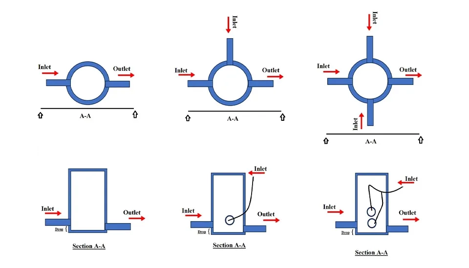
The purpose of a drop manhole is to reduce the turbulence in the manhole if the elevation difference between incoming and outgoing sewers is greater than 1.5 ft (0.5 m). The turbulence caused by a sudden drop of wastewater may cause splashing and release corrosive and odorous gases, and can damage the manhole.
3.2.7. Hazen-Williams Coefficients
Hazen-Williams coefficients are used to calculate pressure drop in pipes; it depends on the quality and condition of the inner surface of the pipe. The amount of this factor is different for new and old pipes. Since the pipe surface may corrode or scale over time, lower values of C should be used in calculations. Therefore, it is important to choose an appropriate value for C depending on the actual conditions of the piping system. It selects the Hazen-Williams coefficients for each pipe from the table below.
A: The C values for new pipes included in the above table are used to determine the acceptability of the surface finish of new pipelines. The user agency may specify that a flow test be conducted to determine the C values of laid pipelines.
B: For pipes of diameter 500 mm and above, the range of C values may be from 90 to 125 for pipes less than 500 mm.
C: In the absence of specific data, this value is recommended. However, in case authentic field data is available, higher rates of up to 130 may be adopted.
Note: Even though the C value can be taken as 145 for Water supply, for sewage, 140 shall be taken for design purposes.
3.3. Design Equations and Procedure
The equations and procedure help designers to optimize the analysis and design the sewage system in the SewerGEMS software. This section continues by defining the proper equations and procedure that affect the design of the wastewater collection system.
3.3.1. Circular Sewer Flowing FulL
Once the peak, average, and minimum flow estimates (including allowances for infiltration/inflow) are made, the general layout and topographic features for each line are established, the design engineer begins to size the sewers. The design equations proposed by Manning, Chezy, Gangrullet, Kutter, and Scobey have been used to design sewers and drains. The Manning equation has received the most widespread application. The Manning equation in various forms is expressed below:
R = hydraulic mean radius= A/P (circular pipe flowing full, R = D/4), m (ft)
A = area of pipe flowing full (π/4 D2), m2 (ft2)
P = wetted perimeter (πD), m (ft)
D = diameter, m (ft)
Q = flow, m3/s (ft3/s)
S = slope of energy grade line or invert slope, m/m (ft/ft)
n = coefficient of roughness used in Manning equation
The coefficient of roughness depends on the material and age of the conduit. Commonly used values of n for different materials are given in the table below.
Table 6. Common Values of Roughness Coefficient Used in the Manning Equation
Material
Commonly Used Values of n
Concrete
0.013 and 0.015
Vitrified clay
0.013 and 0.015
Cast iron
0.013 and 0.015
Brick
0.015 and 0.017
Corrugated metal pipe
0.022 and 0.025
Asbestos cement
0.013 and 0.015
Earthen channels
0.025 and 0.030
3.3.2. Circular Sewer Flowing Partially Full
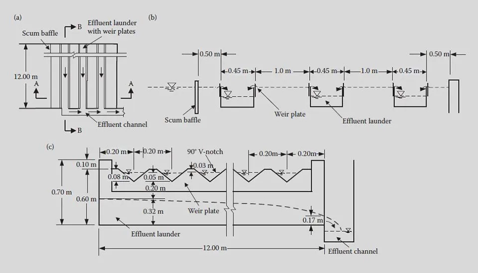
Sanitary sewers are primarily designed to flow partially full. The hydraulic element equations for circular pipe flowing under part-full flow conditions are given by Eqs. (5) and (8) and are graphically shown in fig. 7. The central angle is ϑ. It may be noted that the value of "n" decreases with the depth of flow (Fig. 7). However, in most designs, n is assumed constant for all flow depths (Mackenzie Leo, 2011).
Also, it is common practice to use d, v, q, a, and p (lowercase) notations for flow depth, velocity, discharge, flow area, and wetted perimeter under partial flow conditions. In contrast, t, D, V, Q, A, and P (uppercase) notations are used for sewer flowing full. A sewer line flowing 80 percent full has a d/D ratio of 0.8 (Chukwulozie et al., 2018).
Cos θ/2 = [1 - 2×(d/D)] (Eq. 5)
A = D2/4 × {( πθ/360) - (sinθ/2)} (Eq. 6)
P = πDθ/360 (Eq. 7)
R = D/4 {1- (360 × sinθ/2Dθ)} (Eq. 8)
Friction head loss in a pressure pipe (force main) can be calculated from the Darcy–Weisbach or Hazen– Williams equation (Equation 9 or 10).
hf = (fL/Dh)×(V2/2g) or hf = (fL/4R)×(V2/2g) (Darcy−Weisbach) (Eq. 9)
hf = 6.82(V/C)1.85× (L/D1.167) (Hazen−Williams, SI units) (Eq. 9)
Fig. 7. The element Property Editor in SewerGEMS, used to define hydraulic and physical input parameters for sewer network modeling.
3.4. Design Calculations
Sewer design is a crucial process for the management of surface water and groundwater, which provides an effective and efficient system for transporting sewage. The junction chamber is a key component used to change the flow direction. In addition, junction chambers help minimize leaks and improve the quality of sewage services. Additionally, one of the crucial aspects is the design of the hydraulic profile that indicates water flow behavior in the wastewater systems. These profiles show information about the velocity, flow, and pressure that help designers and engineers develop effective wastewater systems.
Step A: Sewer Design
The design computations for the sewers should be started from the upper reach of the line and carried downward in the direction of the flow.
The cumulative flows between manholes are used to determine the sewer diameter, slope and ground and invert elevations. However, the calculations for only the last section of these pipes are given regarding the floor elevation of the rack chamber. This elevation was established from the old sewer line serving the existing aerated lagoon. The design procedure involves the following steps:
1. Select the diameter, slope, and roughness coefficient n for the sewer line.
2. Determine the discharge Q and velocity V from Eqs. (1) and (2) or from fig. 8 when the sewer is flowing full. Q should be larger than the peak design flow (jica, 2012).
3. Calculate q/Q ratios at peak design flow and minimum initial flow.
4. Determine d/D and v/V ratios at these flows. from fig. 7.
5. Calculate the velocity and depth of flow under these flow conditions.
6. The velocity at minimum initial flow should be greater than 0.45 m/s.
Step B: Junction Chamber
The junction chamber has different internal dimensions that depend on the incoming pipes in it. Three incoming sewers join at the junction chamber. A single line carries the total flow to the treatment facility. A manually operated sluice gate is provided to close the line and divert the flow into the bypass sewer. The bypass sewer is designed to divert the incoming flow into the storage basin at the time of power outages.
Step C: Hydraulic Profile
The water surface profiles for all sewers were developed based on the water depth, slope of the sewer, and head losses encountered in the appurtenances. The head losses in a manhole or collection chamber are caused by (1) exit loss, (2) change in direction, (3) contractions and expansions, (4) transitions, and (5) entrance loss. All these losses may be conveniently expressed by Eq. (5) (Manual on Sewerage and Sewage Treatment):
hL=k(v2/2g) (Eq. 9)
where
hL = minor loss due to entrance, exit, or change in direction of the flow, m
v = velocity of flow, m/s
g = acceleration due to gravity, 9.81 m/s2
K = head loss coefficient
Where k is a bend coefficient, which is a function of the ratio of the radius of curvature of the bend to the width of conduit, deflection angle, cross-section of flow, Reynolds number, and relative roughness.
kb is approximately equal to 0.4 for 90 degrees and 0.32 for 45 degrees and can be linearly proportioned for other deflection angles.
4. The Steps of Designing by SewerGEMS Software
The steps of designing include various methods, creating a new project, importing the entering data, setting the hydraulic features, the analysis system, the optimizing system, generating the report and map, design review and approval, and saving the project to share it with other designers.
The designers can use the capabilities of the SewerGEMS software for designing a system that is effective and stable.
In the next, each method will be provided further explanation.
4.1. Preparation of SewerGEMS Software
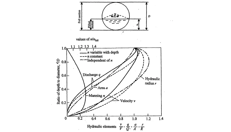
In the first step, selecting the unit for use in SewerGEMS is essential. The software has two units, SI and US customary. For this project, US customary units must be selected. To select this unit, follow the steps in Fig. 8.
First, select ’More’ in the ’Tools’ menu, then choose ’Options’. On the next level, open a window with the name Option, and after that, select the unit US customary in the unit part. However, there may be other cases manually in the list related to the units.
Fig. 8. Sewer system optimization view showing key performance indicators (KPIs) for comparing alternatives in urban wastewater management.
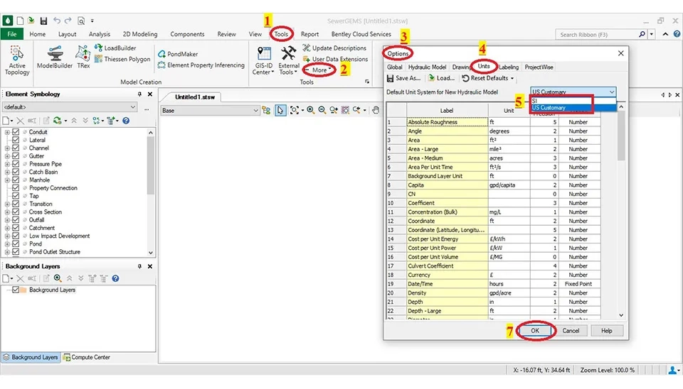
Designers can also select or change the software’s color scheme. To do this step, in the 'Global' section of the options window, they can choose or change the color scheme in the 'Color' window. The color scheme includes colors related to the Background, Foreground, Selection, Read-only Background, and Read-only Foreground (fig. 9). The widely used is the Background and Selection in the SewerGEMS software.
Fig. 9. Creating a new alternative in the SewerGEMS Manager, essential for comparative wastewater system design analysis.
4.2. Adding The Map of The Study Area to Software
Adding the map is essential for drawing the conduits, pipes, manholes, pressure junction, pond, pump station, wet well, outfall, and similar items in SewerGEMS software. There are some ways to add a map to the software.
The first way is to draw pipes, manholes, and other things in Google Earth with KML/kKMZ format and then convert them into (*.shp) format with ArcGIS software or Global Mapper software. In addition, it can add these details to the software from ModelBuilder. This method was done in the Design and Analysis of Water Distribution Network Using WaterGEMS (part 3.1.3).
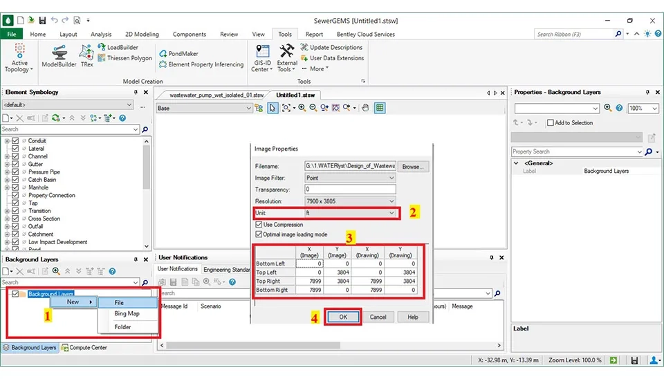
The second way is to use a picture with .TIFF file, it is essential to save a picture with an appropriate format of the study area from Google Earth. Also, it needs to note three or four different UTMs of the study area from Google Earth for the Georeferencing of the picture in Global Mapper. Finally, it has to add the . TIFF file to the SewerGEMS software through the Background Layer in the software (fig. 10).
It is necessary to do the below ways to add .TIFF file from Background Layers. The first, importing .TIFF file was saved on your computer (1-way). Then, it needs to opt for a proper UNIT (2-way). Next, import the UTM (3rd way), coordinates that must be exported from ArcGIS software (Fig. 10).
Fig. 10. Visualization settings for GIS-based sewer design, enabling thematic mapping of results for sewer system optimization.
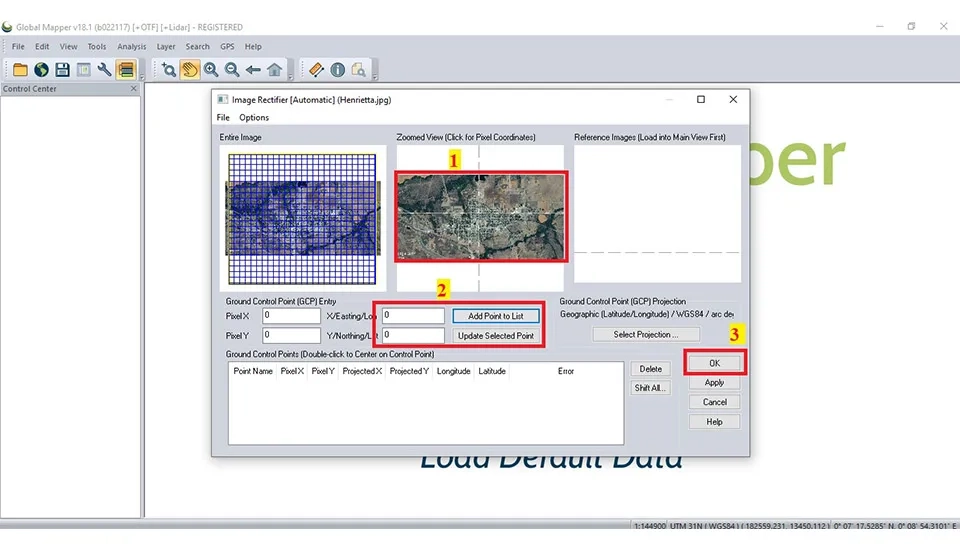
To georeference the picture of the study area, use the Global Mapper as follows:
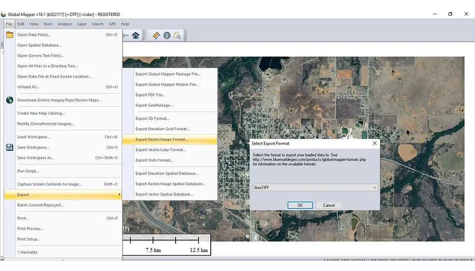
First, add the picture saved from Google Earth on your computer to Global Mapper. Next, import the UTM coordinates that were recorded for the georeference of the picture. Then, click on 'OK' after importing 4 or 3 UTMs (fig. 11). Finally, it needs to save the picture in TIFF format (Fig. 11 and 12).
Option 1: Fig. 11. Creating the color-coding ranges within the Element Symbology manager for visualizing wastewater system design performance in SewerGEMS.Fig. 12. Selecting data fields for a report template, essential for verification and sewer system optimization documentation.
Finally, we can use ArcGis to explore information and get a background in SewerGEMS software. The ways to gain this information from ArcGis are in fig. 13.
Fig. 13. Final output of the Custom Report viewer in SewerGEMS, showing selected data fields for wastewater system design documentation.
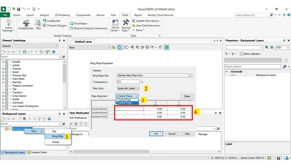
The third way is to add the pipes and manholes using the Bing Map Properties in SewerGEMS. This method offers an online map from the Bing Site, allowing the user to draw the pipes and manholes in the software. To draw the pipes and manholes as follows below:
First, right-click or click the New toolbar button and choose Bing Maps, which opens the Bing Map Properties window. Next, choose between the following three background display styles in Map Style: 'Aerial', 'Aerial with Labels', and 'Road'. The default setting is Road. Then, select 1 or 3 control points from Map Alignment that use 3 control points to cause increased accuracy. Finally, import the latitude and longitude of the map area; also, it can use Google Earth software to access the latitude and longitude of the map area (Fig. 14).
We will use the third method to draw the pipes and manholes in this project.
Fig. 14. The Graph Manager in SewerGEMS displaying a time series plot of results, key for hydraulic simulation and transient analysis.
4.3. Drawing The Major Pipes and Sub-pipe
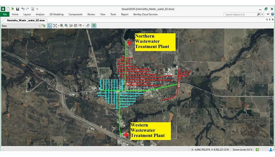
Due to the existence of two wastewater treatment plants in the north and west of Henrietta city, two major pipes must be drawn for moving wastewater to the wastewater plants. Therefore, the city needs to be divided into two parts for drawing the major pipes and sub-pipes (Fig. 15).
Fig. 15. SewerGEMS training: Exporting the GIS-based sewer design network data to DXF, a final step for plan production.
We directly draw the major pipes and sub-pipes through the third method in SewerGEMS. It uses the conduit and manhole elements in the layout part to draw pipes and manholes in SewerGEMS software (fig. 16).
Fig. 16. Finalized sewer profile view in CAD, exported from SewerGEMS and used for detailed wastewater system design documentation.
4.4. Dividing of Wastewater Flow
In this step, the sewer flow must be divided and assigned in SewerGEMS. There are some methods to divide the sewer in the SewerGEMS software.
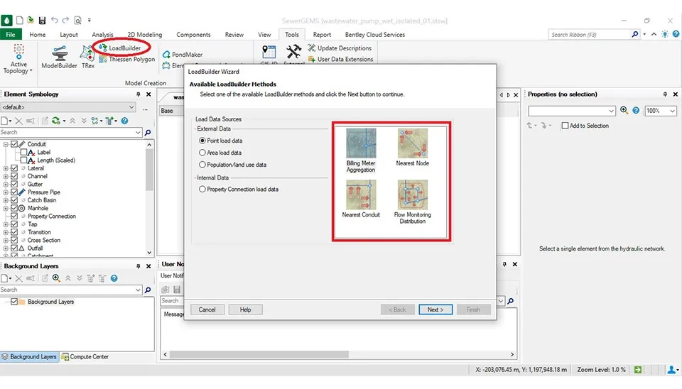
1. Using LoadBuilder to import external data in the SewerGEMS Software
LoadBuilder is a tool to assign flows to each element in Bentley SewerGEMS CONNECT. The power of LoadBuilder is that it can take loading information from a variety of GIS-based sources, such as customer meter data, system flow meters, or polygons with known population or land use, and assign those flows to elements. LoadBuilder is suited for the types of data available to describe dry weather flows, while other methods in Bentley SewerGEMS CONNECT are more amenable to wet weather flows. It includes some ways, as follows:
Billing Meter Aggregation
Nearest Node
Nearest Conduit
Flow Monitoring Distribution
Fig. 17. The Element Symbology dialog open to the Annotation tab, used to define labels for wastewater system design elements in SewerGEMS.
2. Using ArcGIS to Manually Calculate the Area of Each Pipe to Divide Flow
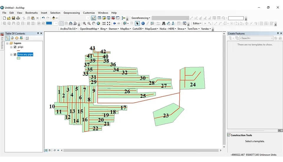
This method needs to convert pipes from the DXF file to format shape (.shp) files. First, it has to export the pipes of SewerGEMS with a DXF file. Clicking on the File in SewerGEMS after selecting Export to save the DXF file on your computer. After that, change the DXF file into a shape (.shp) file with the Global Mapper. Then, import the shape file to ArcGis. Next, calculate the area of each pipe for dividing sewage in the SewerGEMS software (Fig. 18). Engineers can refer to the following link on how to calculate the area and divide the sewage in ArcGIS.
Fig. 18. Customizing the output parameters for the longitudinal sewer profile view, essential for wastewater system design documentation in SewerGEMS.
Finally, it can calculate the wastewater flow based on the area of each pipe divided by the total area of the service for each manhole in the table below. The total area is about 8.742 square miles. Also, total wastewater flow is 47.58 gal/s. For complete data and detailed calculations, refer to Full Table of Caulation Wastewater Flow
Table 7. Calculation of wastewater flow for designing
4.5. Importing The Sewage Flow to Each Manhole Manually
In this way, the Inflow (Sanitary Loading) and Wet Weather Inflow must be imported manually.
The Inflow (Sanitary Loading) is calculated, and the Wet Weather Inflow is estimated based on the Inflow (Sanitary Loading). Therefore, the total wastewater flow in this project is calculated as the sum of Inflow (Sanitary Loading) and Wet Weather Inflow. It can import this calculation through two ways in the SewerGEMS software as follows below. However, the second way will be used in this project for importing wastewater for designing.
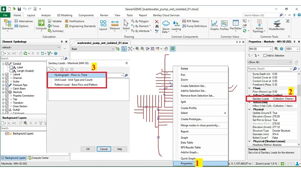
4.5.1. Inflow (Sanitary Loading)
1. Click a node element in your model to display the Property Editor, or right-click a node element and select Properties from the shortcut menu.
2. In the Inflow Collection section of the Properties, click the Ellipses (...) button. The Inflow Collection Editor appears.
3. Click the New button, then select the type of inflow you want to create from the submenu (Fixed Inflow, Hydrograph Inflow, Pattern Inflow).
4. For a hydrograph inflow, enter the data points in the hydrograph table. For fixed and pattern inflows, enter the data in the appropriate fields. For a hydrograph, if the last time in the table is less than the total simulation time, the simulation time and last flow will be appended to the hydrograph table.
5. Repeat steps 3 and 4 for each inflow you want to add to the collection.
6. Click the Composite Hydrograph button to see a graph of the composite hydrograph.
7. Click the Composite HydrographData Table button to see a tabular view of all the data points in the composite hydrograph.
8. Click OK to close the dialog box and add the collection data to the Property Editor.
Fig. 19. Selecting data fields for the customized longitudinal sewer profile output, key for wastewater system design documentation in SewerGEMS.
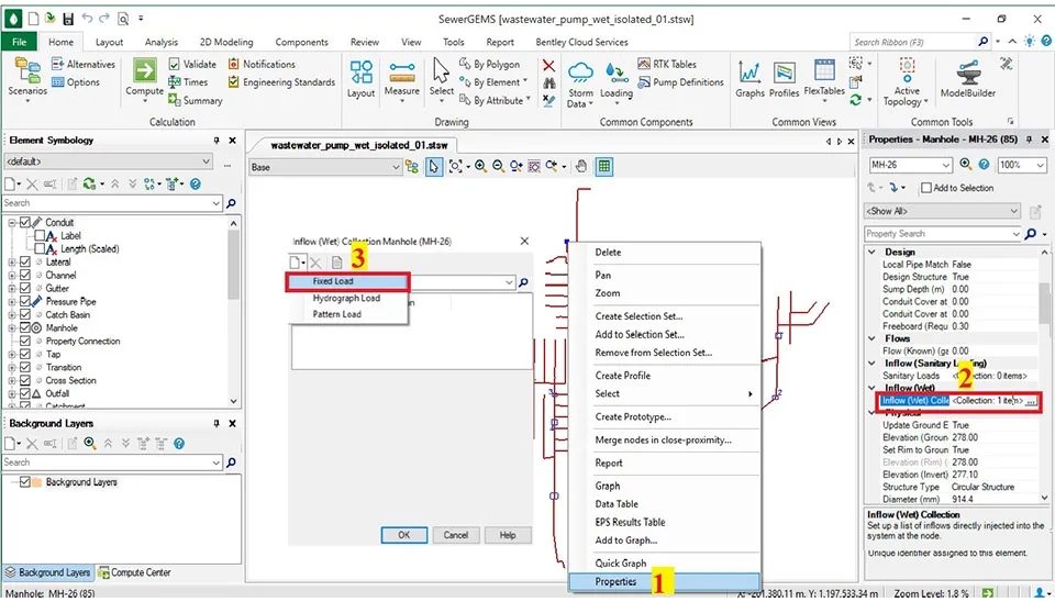
4.5.2. Inflow Wet Collection
The Wet Weather Inflow is used when the wastewater flow is calculated by Fixed Inflow. We also calculated the wastewater flow by Fixed Inflow in the table above.
For importing wastewater, it follows ways below (Fig. 20):
1. Click a node element in your model to display the Property Editor, or right-click a node element and select Properties from the shortcut menu.
2. In the Inflow Collection section of the Properties, click the Ellipses (...) button. The Inflow Collection Editor appears.
3. Select the fixed load, and open a box with the fixed load.
Fig. 20. SewerGEMS training: The final, customized profile output in DXF format, used for comprehensive sewer network modeling documentation.
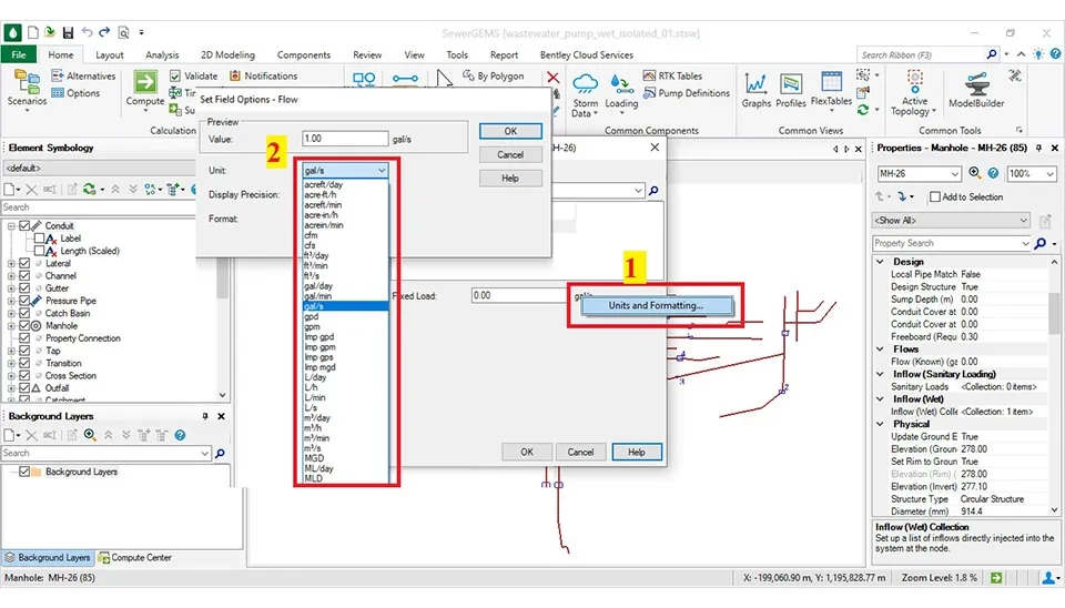
Subsequently, the unit suitable for the project must be chosen, selecting the gal/s unit for this project, as shown in Figure 21.
1. First, right-click in front of the box that imports the inflow and choose Unit and Formatting.
2. Then, open a window named the Set Field Option Flow. It needs to set the unit, display precision, and format in this box. In order, the unit is set with the proper unit for designing, display precision is set with one or two decimal places, and, format is set with number.
Fig. 21. Section of the final hydraulic design profile exported from SewerGEMS, ready for submission in the wastewater system design package.
4.6. Importing the Information Suitable Diameter of Pipe for Wastewater Flow
There are several different pipes available for wastewater collection systems, each with unique characteristics that are suitable for different conditions. The four different pipes widely used are ductile iron, concrete, plastic, and vitrified clay.
Manufacturers of these pipes need to follow requirements set by the American Society of Testing Materials (ASTM) or American Water Works Association (AWWA) for specific pipe materials. These standards cover the manufacture of pipes and specify parameters such as internal diameter, loadings (classes), and wall thickness (schedule). The methods of pipe construction vary greatly with the pipe materials.
The advantages and disadvantages of specific pipe materials are listed in the table below. The primary advantages and disadvantages to consider for pipes used in sewer applications include those that are related to construction requirements, pressure requirements (force mains), depth of cover, and cost (EPA, 2000).
Table 8. Advantages & Disadvantages Of Different Materials
Advantages
Disadvantages
Ductile Iron
Good corrosion resistance when coated
High strength
Heavy
Concrete
Good corrosion resistance
Widespread availability
High strength
Good load-supporting capacity
Requires careful installation to avoid cracking
Heavy
Susceptible to attack by H2S and acids when pipes are not coated
Short length and numerous joints make it prone to infiltration and more costly to install
Thermoplastics (PVC, PE, HDPE, ABS)
Very lightweight
According to the table above, the best quality and most widely used is the type of pipe generated by PVC, PE, HDPE, and ABS. Therefore, it chose the PVC pipe for this project.
4.6.1. Calculation of Pipe Diameter
It needs to calculate the pipe diameter for each pipe according to Eqs. 3 to 9, also, 80 percent occupancy should be considered. This step calculates the diameter for the divided maximum wastewater flow for a pipe available in this project.
The first step is calculation of diameter from Equation 4 (Q= 0.464/n × D8/3 × S1/2 ) By default, the minimum slope for the pipe with a diameter of 150 mm is used in this equation:
Note: if the diameter of the pipe is calculated to be between two recommended diameters, it is necessary to select the higher diameter For example, if the pipe diameter is calculated as 8.5 inches, which is between 8-inch and 10-inch diameters recommended, so; it will prefer the pipe with a 10-inch diameters.
The next step is to check the velocity in this pipe (D = 6 inch):
Cos θ/2 = (1- (2d/D)) ⇒ d/D=0.8 ⇒ Cos θ/2 = (1- 1.6) ⇒ θ/2=cos−1 (−0.6) ⇒ θ = 254.4∘
A = D2/4 × {( πθ/360) - (sinθ/2)} ⇒ A = D2/4 × {( π×254.4∘/360) - (sin254.4∘/2)} ⇒ A = 0.613×D2
P = π×D×θ/360 ⇒ P = π×D×254.4∘/360 ⇒ P = 2.2217×D
R = D/4 {1- (360 × sinθ/2×D×θ)}⇒ R = D/4 {1- (360 × sin254.4∘/2×D×254.4∘)}⇒ R= (D/4)+0.0818
The calculation of the pipe velocity is as follows (D = 0.504 ft):
V=1.486/n × R2/3 × s1/2 ⇒ V = (1.486/0.009)×[(0.504/4)+0.0818]⅔ × 0.0061/2 ⇒ V = 4.46 ft/s
Note: If the calculated velocity in the pipe is not within the appropriate range, we first change the slope of the pipe to achieve the proper diameter and then we can change the diameter. Also, velocity is directly related to the slope. The higher the slope, the higher the velocity in the pipe; unlike, the lower the slope, the lower the velocity in the pipe.
According to the minimum velocity of 1 ft/s (0.3 m/s) and the maximum velocity of 3.28 ft/s (1.0 m/s), the velocity of this pipe (D = 0.504 ft) is in the proper range, therefore the pipe is suitable for design; alike, these equations can be used to calculate the diameter of the remaining pipes.
4.6.2. How to Enter The Main Information of Each Pipe in The Wastewater Software
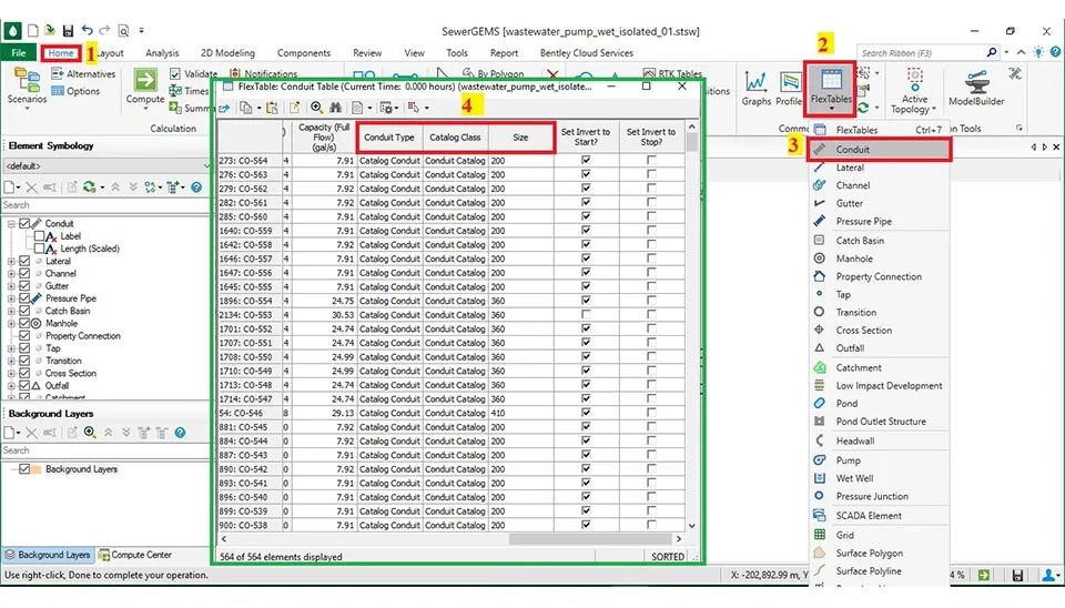
The main information for each pipe includes the conduit type, size, section type, material, wall thickness, Manning’s n, slope invert, invert start, invert stop, and slope.
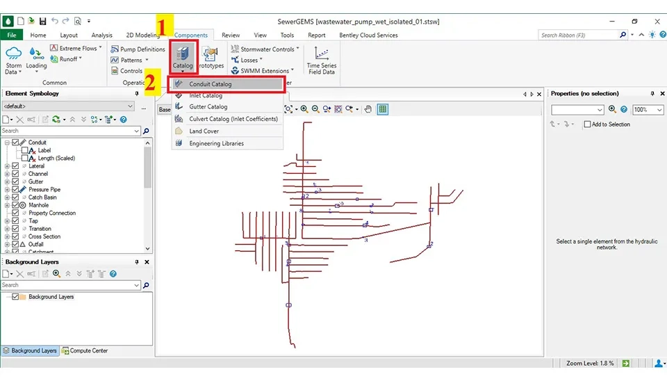
One of the advantages of this software is that it can create a catalog containing information that does not need to be imported individually for each pipe.
Initially, it needs to click on the Catalog in the components part (step 1). Then, selecting the conduit catalog opens a new window that includes the material, diameter, Manning’s and Hazen-Williams factors, and wall thickness for each material (step 2).
Fig. 22. Finalized sewer network plan view in CAD, showing the layout and labels, ready for wastewater system design submission.
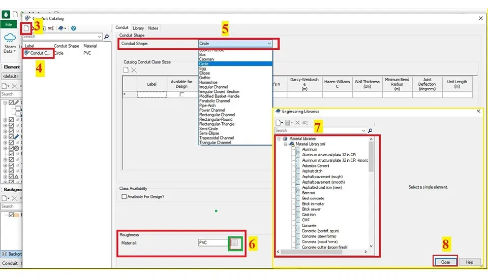
In the step, click on "New" in Step 4 to write a name for this catalog, then, select kind of the conduit shape (step 5). Also, choose the type of material in the roughness (step 6). Therefore, select the pipe desired (step 7), and finally, click on the close (step 8).
Fig. 23. Detail of the finalized sewer network plan view in CAD, displaying required data and labels for wastewater system design.
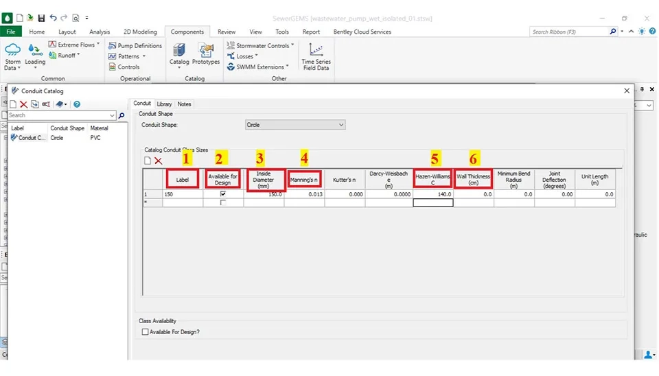
Finally, a table should be completed, which requires steps 1 to 6 in Fig. 24 to write the wall thickness (step 6) when using a pipe whose outside diameter must be written in the table, such as a polyethylene pipe.
Fig. 24. Sanitary Load Control Center in SewerGEMS, used to input and manage flow demands for wastewater system design.
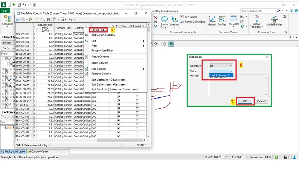
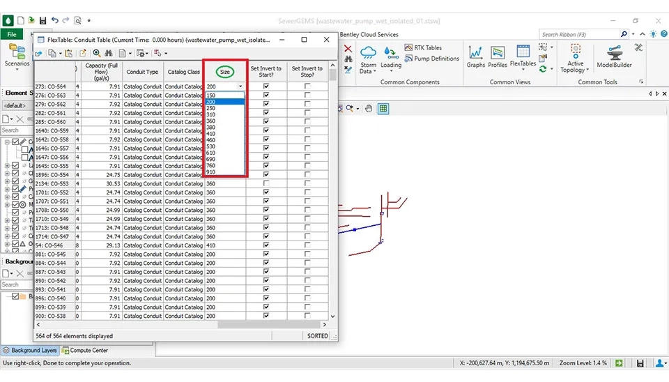
Now, there is a table with some information that it is possible to import data of a pipe or a group of pipes with a similar size. There are two methods to import the data from this table, for each pipe or a group of pipes with similar diameters.
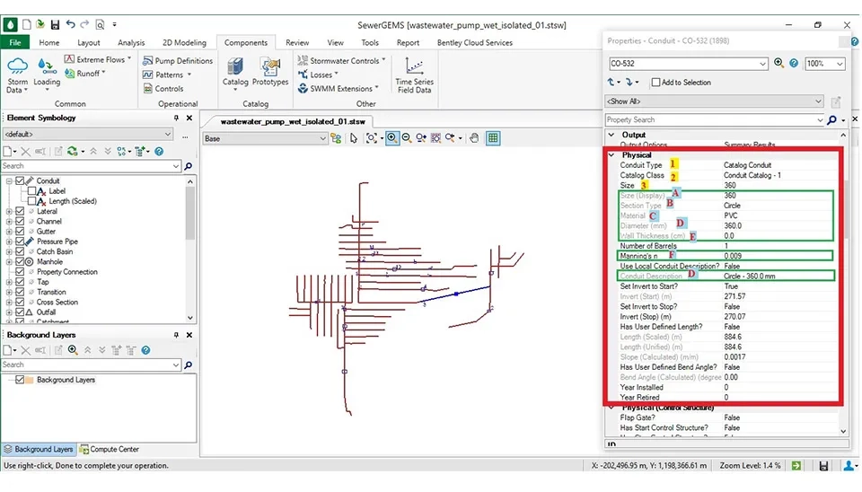
The first method is to double-click on a pipe in the main window of the software, or right-click on the pipe and Select "Properties". Then, it opens a window with the properties-conduit.
In the first step, choose the catalog conduit that was created in the previous step; also, in the second step, select the table materials for each pipe that was made in the previous step. In the third step, the pipe size is selected for the selected pipe or group of selected pipes.
When they are done with the steps above, the Size (Display), Section Type, Material, Diameter, Wall Thickness (mm), Manning’s, and Conduit Description are chosen automatically.
Note: It can only change Manning’s factor in this table; to change other items, you need to refer to the main table.
Fig. 25. Inputting unit loads and allocation factors in the SewerGEMS Load Editor, crucial for accurate wastewater system design.Fig. 26. Table detailing the input of sanitary flow demand patterns and factors for accurate wastewater system design in SewerGEMSFig. 27. Data grid detailing demand allocation of sanitary loads, a key step for wastewater system design and flow analysis in SewerGEMS.Fig. 28. Graphical view of the sanitary flow demand pattern or diurnal curve used for wastewater system design in SewerGEMS.Fig. 29. Data grid showing the resulting demand allocation of flow loads after applying patterns, vital for wastewater system design.
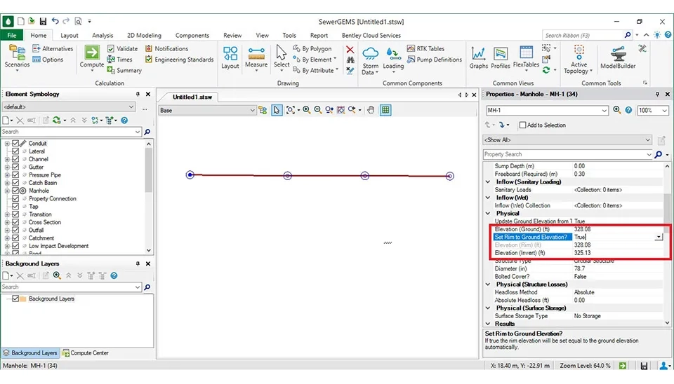
4.7. Detail of Each Manhole
The main details of each manhole include the ground elevation, the rim elevation, and the invert elevation. The ground elevation usually shows the ground elevation for the current locations. In addition, the information on the elevation ground should be imported for this item. Besides, the rim elevation is typically flush with the ground surface. The invert elevation shows the depth of the manhole relative to the ground elevation.
4.7.1. The Placement of each Manhole in Wastewater Software
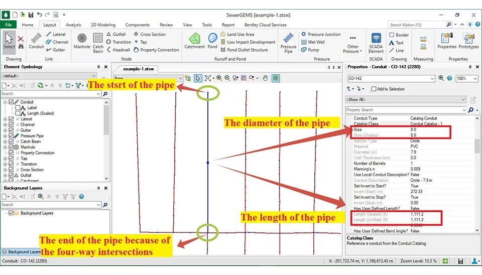
The distance of each manhole depends on the diameter of the pipe. Therefore, to select the suitable distance for the manhole, refer to the Table related to the distance between manholes (Part 3.5.2). In this article, we will initially use a pipe with a diameter of 8 inches (200 mm). Accordingly, the distance between the two manholes will be 148 ft (45 m). However, in last level, it will be calculated a proper pipe for each flow, also, it can be estimated the pipe by trial and error in the SewerGEMS Software. Meanwhile, it must be imported into the software before placing the manholes.
There is a main point to creating manholes in the software that is crucial to creating manholes equally. For example, there is a pipe with every length. The distance of the pipe must be divided into the distance between two manholes, which is determined by the diameter of the pipe. Finally, the result will be used for the distance between two manholes in the SewerGEMS software.
You can follow the step below as an example:
The length of pipe is ⇒ L= 1111 ft (338.5 m).
The diameter of pipe is ⇒ D= 8 inch (200 mm).
And the distance of two manholes should be 148 ft (45 meters) because of the diameter. So;
The number of manholes is ⇒ N= L length ofpipe / L distance of two manholes⇒ 1111/148= 7.5 ⇒ N = 8 ⇒L distance of two manholes=L length ofpipe/N ⇒ 1111/8=138.8ft⇒L distance of two manholes=140 ft (43 meters)
Therefore, it must be the distance between two manholes of 140 ft (43 m).
This method is for situations where the pipe is straight, so wherever the pipe path changes, it is needed to create a manhole, such as at intersections, four-way intersections, or three-way intersections. Hence, these areas will be the end of the pipe to calculate the distance between manholes.
Fig. 30. Final data grid showing the calculated demand allocation of sanitary loads, verified for wastewater system design in SewerGEMS.
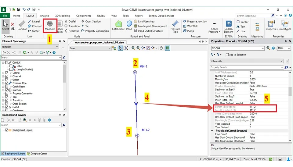
For importing manholes in the SewerGEMS software, follow the below steps:
Initially, it is selected on the manhole in the layout part of the SewerGEMS software, then clicked on the pipe desired for creating the first manhole. Next, it is estimated at a distance and creates a second manhole. Therefore, clicking on the pipe between two manholes is created to check the distance; if the distance is lower or more than the distance desired (148 ft), it can move the second manhole to find the distance suitable. Thus, it can be done for creating other manholes in the software (fig. 31).
Fig. 31. Graphical review of the sanitary flow demand pattern or diurnal curve used for wastewater system design in SewerGEMS.
4.7.2. Import The Main Information each Manhole in Wastewater Software
After dividing a pipe for placing manholes, it is necessary import some information for each manhole. Thus, each manhole has a minimum of one input pipe or a maximum of three input pipes. Also, it has an output pipe that has to be more down than other pipe inputs in order in terms of elevation because the flow moves gravitationally (Fig. 32).
Fig. 32. Output table summarizing hydraulic simulation results, including pipe flow, velocity, and HGL for wastewater system design.
The Ground Elevation and The Invert Elevation will be imported for the first manhole and the flow from the manhole manually. But the next manholes automatically get the elevation of the lowest input pipe into a manhole plus a drop as the invert elevation. This condition is continued until the elevation of the manhole reaches the maximum elevation, about 20 ft. Then, The invert elevation has to go up until about the 3 ft ratio The ground elevation, which means that this area needs a wet well and a pump station. The next levels will describe the design of the wet well and pump station.
1: Fig. 33. Output table summarizing hydraulic simulation results, including pipe diameter, velocity, and HGL for wastewater system design.
4.7.2.1. Maximum Invert Drop Across Each Manhole
The maximum invert drop across a manhole for sewers 15 inches (3.8 m) in diameter and smaller shall be 0.60 feet (18 cm) for straight-through flow and 1.00 feet (30.5 cm) for side inlet flow (Sewer Design Guide, 2015).
Table 9. Invert Drops Across Manholes
Diameter of
Outlet
(inches)
Diameter of Inlet (inches)
Inlet Drop to be added (feet)
8
10
12
10
0.08
—
—
12
0.17
0.08
—
15
0.29
0.21
0.13
18
0.42
0.33
0.25
Fig. 34. Output table summarizing hydraulic simulation results, showing final flow, velocity, and pipe properties for wastewater system design.
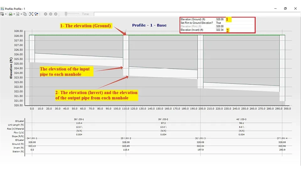
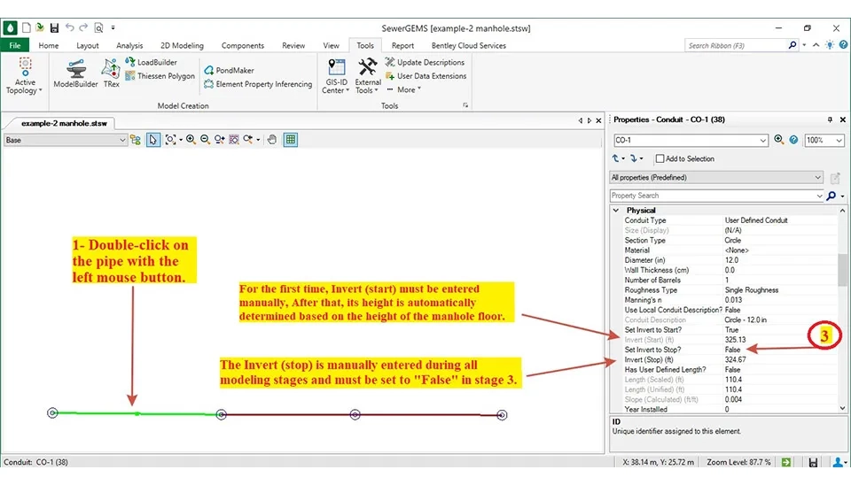
4.8. How to Calculate The Slope of Each Pipe Between Two Manholes
The Invert (Start) and Invert (Stop) are the main information to calculate for each pipe. The Invert (Start) will be gotten automatically from the elevation of the input of the manhole because both of them are the same elevation in design if "Set Invert to Start" is ‘’True’’. But the set invert stop needs to be ‘’False’’ in order for the Invert (Stop) to be calculated before manually importing the elevation. Therefore, the three factors needed are the Invert (Start) elevation, the length of the pipe, and the suitable slope in the table “The Minimum Recommended Slope of Sanitary Sewer” (Part 3.2.3). (part 3.2.2). It needs to choose the suitable slope based on the diameter of the pipe.
The formula for calculate the slope for pipe 8 inch (200 mm) is as follows below:
Slope = The Invert (stop) - invert (start)/ length of pipe ⇒
The Invert (stop) = The invert (start) - (length of pipe × Slope) ⇒
Slope for the pipe with 8 in: S= 0.004 ft/ft
The length of the pipe: L= 110.4 (ft)
The elevation of the Invert (start): Ela= 325.13 ft
The Invert (stop) = 325.13 - (110.4*0.004) ⇒ 324.69 ft ⇒ The Invert (stop)= 324.69 ft
Therefore, this method must be done for all pipes before designing.
Fig. 35. Profile of a sewer pipe in SewerGEMS, used to visualize flow conditions and verify wastewater system design performance.
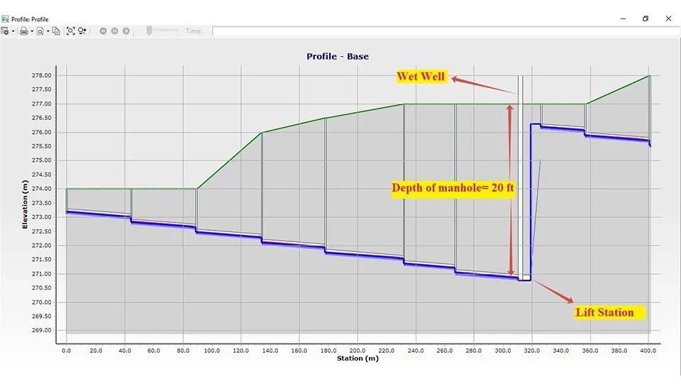
4.9. The Lift Station
When the depth of the manhole is more than about 20 ft (6 meters) in design, it needs to use a lift station. So that the sewage of the manhole can enter the wet well, then a lift station will be used, and the sewage will be transferred to a manhole that has a height of 3 ft (0.9 m) relative to the earth. Again, all method calculations will be done for this manhole, other manholes, and pipes until the depth of the manhole is taken to be more than about 20 ft (6 meters).
To import the wet well and lift station, you need to select the wet well and pump in the layout in the SewerGEMS software. The conduits that connect the wet well to the pump and the pump to the manhole must be changed by right-clicking on the conduit and selecting 'Morph Pressure Pipe to Conduit' (fig. 36).
Fig. 36. Profile of a sewer pipe, used to visualize flow conditions and verify final wastewater system design performance.
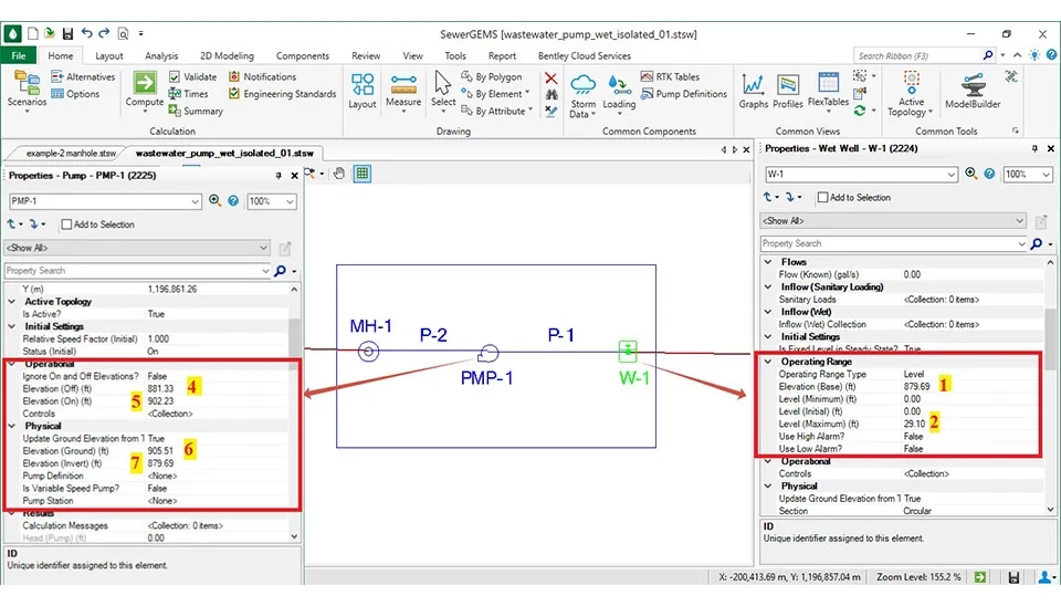
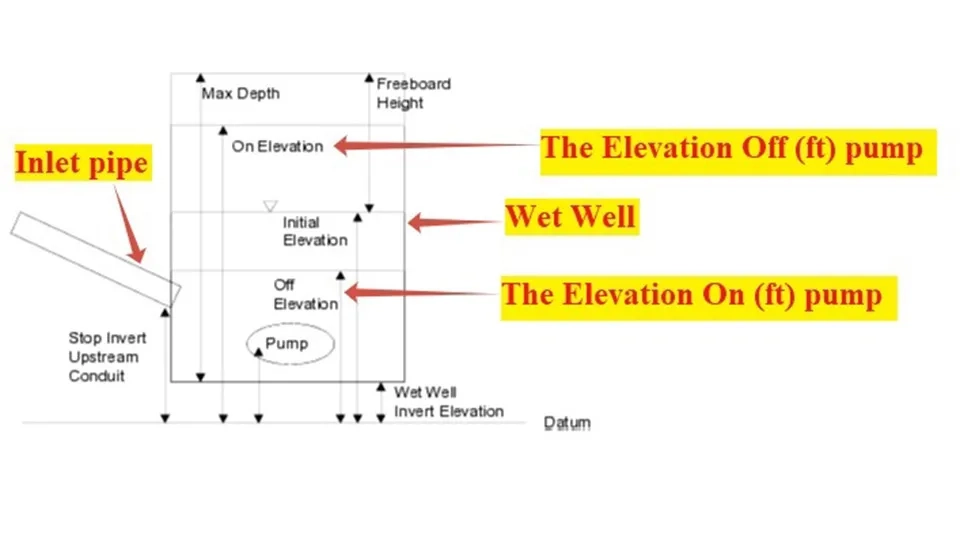
The Base Elevation (ft) and the Maximum Level (ft) are the main information needed for each wet well. The elevation (base) (ft) can equal the elevation of the last manhole. Also, the level (maximum) (ft) can be equal to the elevation of the earth or more to avoid entering the surface water of rain into the wet well.
The lift pump may include one or more pumps that move sewage from the wet well to the highest-level manhole. Thus, the pump-on and pump-off elevations (ft) are the main data required for any pump in a lift station(Fig. 37).
Fig. 37. Longitudinal profile view of a pipe segment showing the hydraulic gradient line (HGL) after the final hydraulic simulation run.
Hence, The Pump-Off Elevation is usually set at a minimum above the inlet pipe's elevation to the Wet Well to prevent air from entering the submersible sewage pumps, which must always be submerged in the wastewater. Therefore, the level switches are used to control on and off these pumps. Conversely, "Pump-On Elevation" (ft) has to be the amount that prevents the overflowing sewage from the wet well at a maximum (fig. 38).
Note: The wet well and the pump are connected by a pressure pipe, which is called an inlet pipe to the wet well. However, the elevation of both the beginning and the end of this pipe should be equal to the bottom elevation of the wet well.
Fig. 38. Plan view of the sewer network in SewerGEMS, color-coded to visualize hydraulic simulation results like velocity or capacity.
Therefore, a lift station is used when the depth of a manhole becomes equal to or more than around 20 ft (6 m) (Fig. 39)
Fig. 39. Graphical review of the sanitary flow demand pattern or diurnal curve used for wastewater system design in SewerGEMS.
Submersible pumps must be used for collecting wastewater in the system. These pumps do not have suction pipes, so it is crucial to link the pumps to a suction node (Wet Well) with a suction pipe (pressure pipe) in the SewerGEMS software design. Thus, The designer needs to utilize a short pipe for connecting the wet well to the pump that ensures minimal head loss (Fig. 40).
Fig. 40. Graphical review of the sanitary flow demand pattern or diurnal curve used for wastewater system design in SewerGEMS.
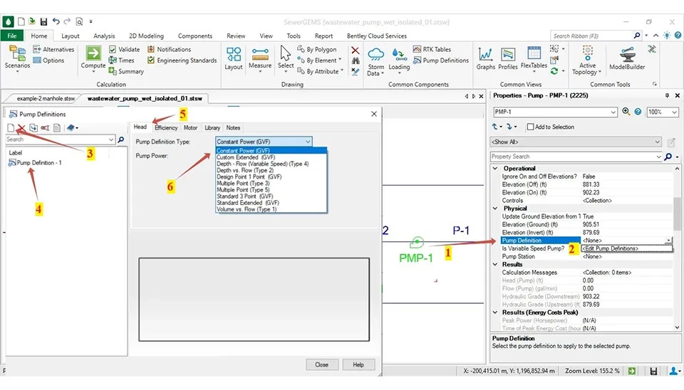
4.9.1. How to Import The Information of The Pump for The Lift Station
There are some methods to import the information of the pump for the lift station. One of them imports a pump based on the flow rate and head; to learn this method, it was done in the Design and Analysis of Water Distribution Network Using WaterGEMS that goes to the following (part 4.8).
Another method is importing the power of the pump into the SewerGEMS software. Initially, it must compute a pump kilowatt based on the flow rate, head, and efficiencies of the pump. The pump output power and efficiency are calculated by Equations 10 through 12.(10-12).
Pw= K’ Q (TDH)γ (Equation 10)
Ep= Pw/Pp (Equation 11)
Ee= Pw/Pm (Equation 11)
Where
Ep= power output of the pump (water power), kW [hp (horse power)]
Pw= power input to the pump (brake power), kW (hp)
Pp= power input to the motor (electrical energy or wire power), kW (hp)
Pm= power input to the motor (electrical energy or wire power), kW (hp)
Q= capacity, discharge, or flow rate, m3/s (ft3/s)
TDH= total dynamic head, m (ft)
γ= specific weight of the liquid pumped, kN/m3 (lb/ft3)
EP= pump efficiency, usually 70-90 percent
EE= pump efficiency, usually 90-98 percent
K’=constant depending on the units of expression
(TDH = m, Q = m3/s, γ = 9.81 kN/m3 , Pw= kW, K' = 1 kW/kN . m/s)
In this article, a pump is delivering 180 GPM at a TDH of 26 ft (7 m). The pump efficiency is 85% and motor efficiency is 92%. Calculate the wire power or electrical energy input to the motor. Use γ = 62.4 lb/ft3 (9.81 kN/m3).
TDH= The ground elevation of The Wet Well - The base elevation of The Wet Well ⇒ TDH= 905.51 - 879.69 = 25.82 ft ⇒ TDH= 26 ft (7 m)
Pw= K’ Q (TDH)γ ⇒ 1/550 hp/ft × 0.4 ft3/s × 26 ft × 62.4 lb/ft3 ⇒ Pw= 1.18 hp
Ep= Pw / Pp ⇒ Pp= Pw / Ep ⇒ Pp= 1.18/0.85 ⇒ Pp= 1.4 hp
Ee= Pw / Pm ⇒ Pm= Pw / Ee ⇒ Pm= 1.18/0.92 ⇒ Pm= 1.3 hp
Therefore, the amount of Brake power input to the pump (Pp) is used in the design (Pp = 1.4 hp).
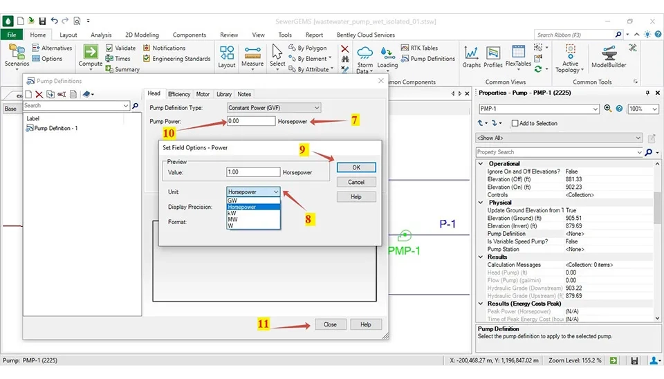
These methods will be used to import the amount of power input to the pump (Pp) in the SewerGEMS software. First, double-click on the desired pump, then open a dialog box where you must click on 'Pump Definition' in the 'Physical' section of this box. Next, it has to select ‘’<Edit Pump Definitions>’’. It opens another dialog box for importing the power of the pump (1.4 hp). After that, it must select on the ‘’New’’ to import a new pump, so, it must opt for the type of the pump in the ‘’Pump Definitions Type’’, and it imports the power of the pump (1.4 hp) in the part of Pump Power. You can change the Unit if the proper is not available. Unit right-click in front of where the pump power is imported to open a dialog box where the unit is changed. Finally, it has to click on the ‘’close’’ as shown in order in the fig.s 41 and 42.
Fig. 41. Graphical review of the sanitary flow demand pattern or diurnal curve used for wastewater system design in SewerGEMS.Fig. 42. Final plan view of the sewer network in SewerGEMS, color-coded to visualize hydraulic simulation results like velocity or capacity.
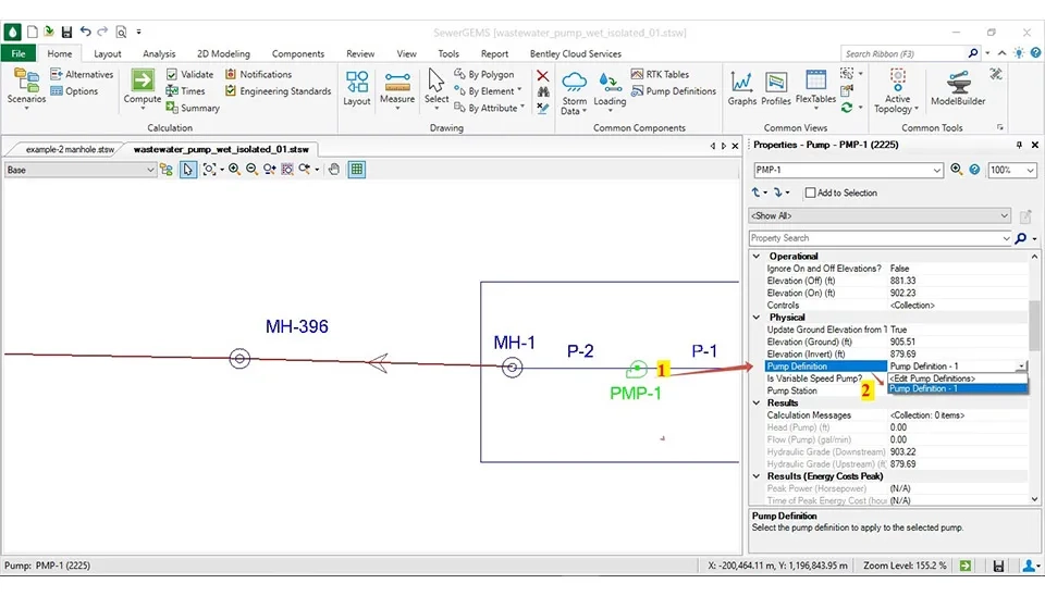
Accordingly, the pump has to choose that import in the software for design. First, double-click on the desired pumps, then open a dialog box that must click on ‘’Pump Definition’’ on the physical part of this box. This is where you will choose the pump needed for design as shown in order in fig. 43.
Fig. 43. Applying the final pump definition to the pump element (PMP-1) properties for accurate hydraulic simulation of the lift station.
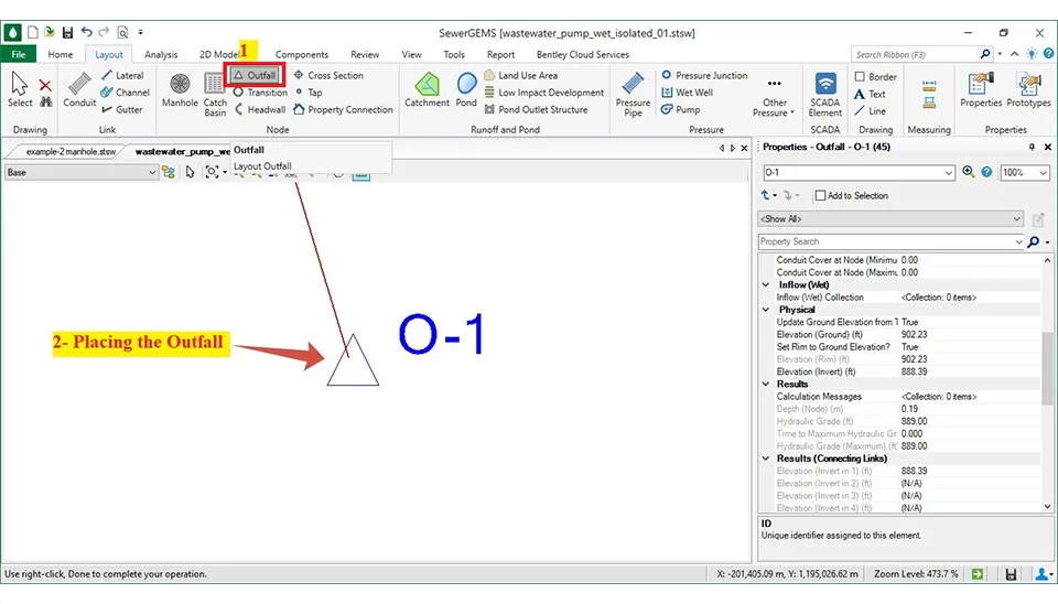
4.10. The Point of Wastewater Discharge in The SewerGEMS Software
The point of the output is called Outfall in SewerGEMS. Placing the outfall is the last step in the design and analysis. To import the Outfall, use the 'Outfall' tool in the 'Layout' section of the software. It is crucial to place the Outfall in the lowest elevation because the wastewater system is by gravity (fig. 44).
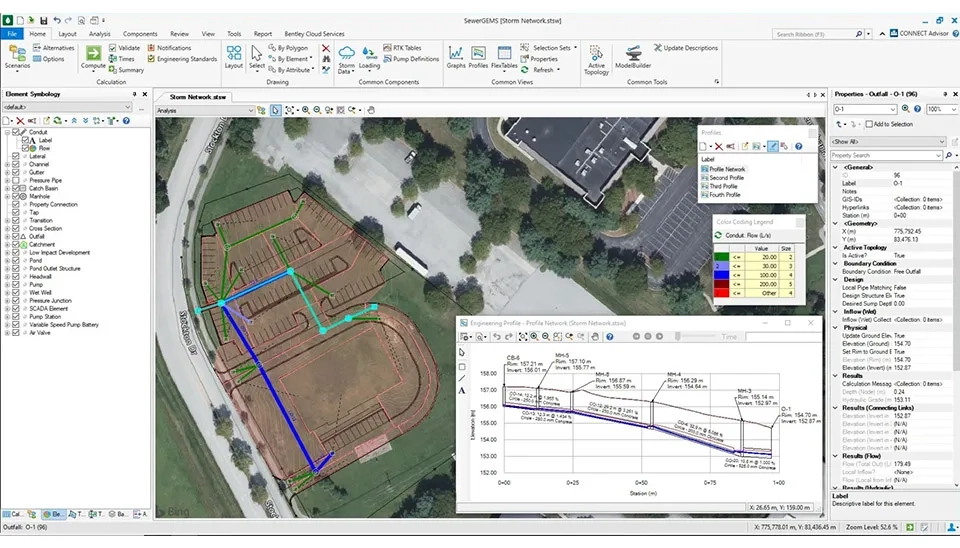
Fig. 44. The final physical modeling step: Placing the Outfall element (O-1) to mark the discharge point for wastewater system design.
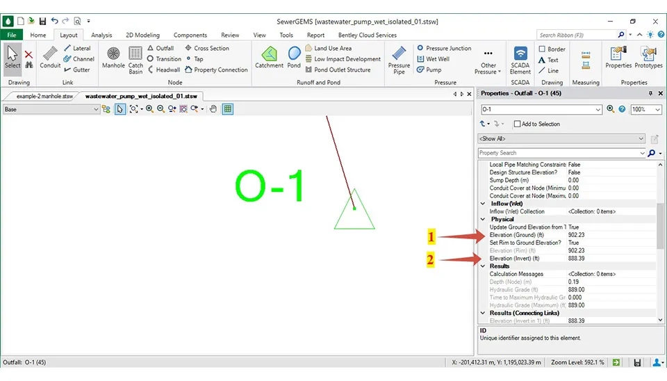
There are two items that have to be imported for each outfall; one of them is the Ground Elevation, which can be equal to the surface elevation or higher to prevent rain surface water from entering the outfall. Another important item is the Invert Elevation, which also represents the lowest point of the hydraulic structure for flow into the wastewater treatment plant. Also, it can check the flow rate in the Outfall that the flow in this area must equal to the flow calculation for initial design (Fig. 45).
Fig. 45. Setting the Ground Elevation and Rim Elevation properties for the Outfall (O-1) to complete the wastewater system design model setup.
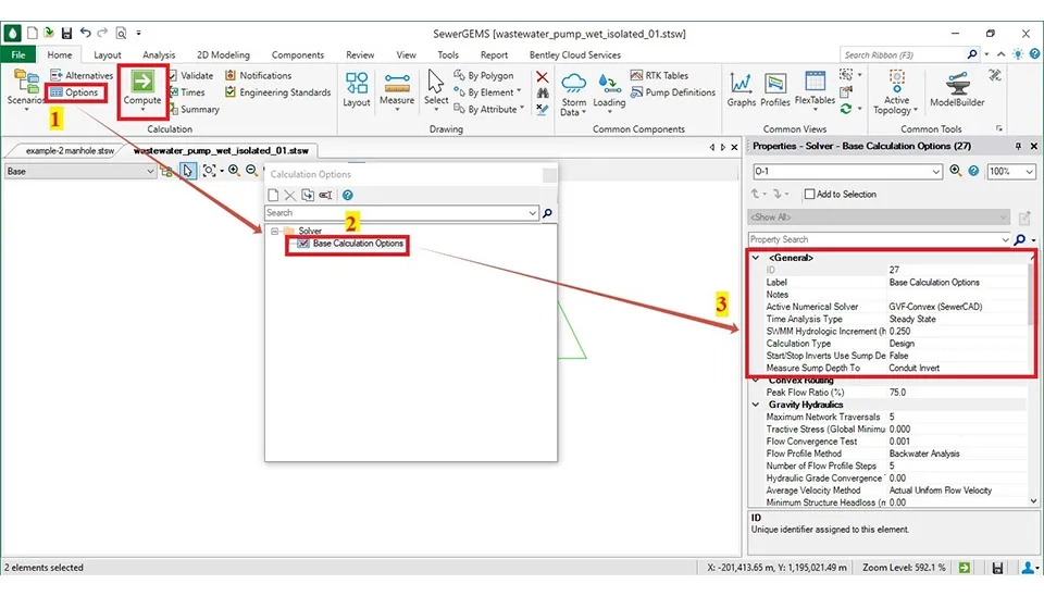
4.11. Opting of The Suitable Numerical Solver for Designing
There are some methods to designin the SewerGEMS software. First, select ‘’Option’’ in the ‘’Home’’ part that opens a dialog box with the name ‘’Calculation Options’’. After that, it chooses ‘’Solver’’ ⇾ ‘’Base Calculation Options’’. Next, it will open a dialog box with the name ‘’Properties - Solver - Base Calculation Options’’ that there are some items in this box that must opt based on the design.
The methods used for the particular items for designing in this article are as follows:
1: "GVF-Convex (SewerCAD) will be selected for ‘’Active Numerical Solver’’.
2. ‘’Design’’ will be selected for ‘’Calculation Type’’.
Therefore , it will be selected ‘’Compute’’ in the SewerGEMS software for designing.
Fig. 46. SewerGEMS training: Setting up the "Base Calculation Options" for the final hydraulic simulation run, including the calculation type and solver.
5. Results
The results include information on the conduits, manholes, lift stations, the outfall, and similar items. The results can be viewed as follows (Fig. 47):
First click the Flex Tables on the Home Part in the SewerGEMS software to see all features of the output of the model. The main items are the conduit is the length of the pipe, the velocity, the slope, and other things. Also, the manhole includes the Rim and the Ground elevation. Additionally, the lift station includes information about each pump (Fig. 47).
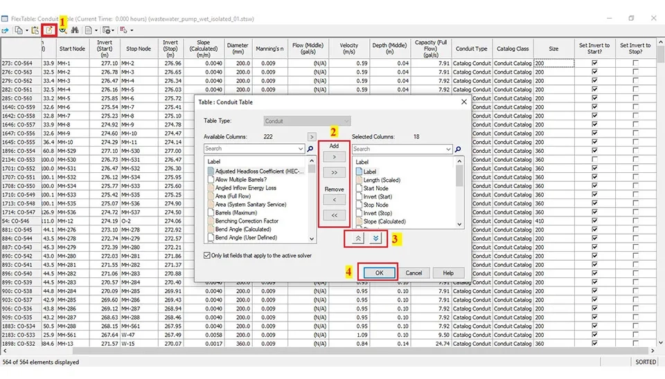
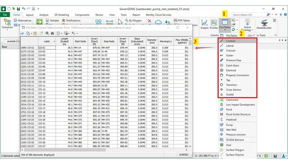
Fig. 47. Accessing the Conduit FlexTable to view and edit large amounts of data, a key step in sewer network modeling and verification.
5.1. The Report of The Pipe
The total length of the pipe was 88,100.9 ft(26853.15 m). Also, numerous pipe diameters were used in this design, from 8 inches (200 mm) to 18 inches (450 mm). The PVC pipe was selected with Manning's n and Hazen-Williams’s C factors of 0.013 and 130, respectively. In addition, the lowest velocity is 0.28 ft/s in the pipe 8 inches, and the most velocity is 3.73 ft/s in the pipe 16 inches.
Table 10. Display the information of the Conduit
Label
Length (ft)
Velocity (ft/s)
Capacity (gal/s)
Manning's n
Hazen-Williams C
CO-1
140.2
1.42
5.71
0.013
130
CO-2
135.9
1.42
5.72
0.013
130
CO-3
111.2
1.93
8.26
0.009
150
Due to the extensive amount of conduit output information, only ten rows are provided here to help engineers become familiar with the pertinent table. For comprehensive information, engineers can refer to Full Table of
There is some information in the reporting of the manhole that helps the designer to analyse and manage the wastewater system. The main information will be described below. The details of the manhole are presented in the table, including the diameter, depth, and type of manhole. Also, the table presents the hydraulic features of each manhole, such as the input and output flow rates, the level of wastewater in each manhole, and the hydraulic pressure.
Finally, the reporting of this information helps in designing to get the best idea of the designing, optimisation, and maintenance. Additionally, these data are important for future planning, evaluating weaknesses, and identifying potential problems.
Table 11. Display the information of the Manhol
Label
Ground Elavation
(ft)
Invert Elevation(ft)
Hydraulic Grade Line (Out)
(ft)
Downstream Conduit Velocity
(ft/s)
Downstream Conduit Flow (gal/s)
Downstream Conduit
MH-1
912.07
909.12
909.26
1.78
0.7
CO-1
MH-2
912.07
898.82
898.96
1.78
0.7
CO-2
MH-3
912.07
896.49
Due to the extensive amount of manhole output information, only ten rows are provided here to help engineers become familiar with the pertinent table. For comprehensive information, engineers can refer to Full Table of Display the information of the Manhole
5.3. The Report of The Lift station
The lift station is one of the main steps in designing and analysing the wastewater system. The lift station will be used to move the wastewater from the lowest place to the highest level. Also, each lift station may have one or more pumps. This system will be used when the depth of the manhole will be more than 20 ft (6 m). The flow and the head are the main factors in selecting a pump. In addition, we choose the pump based on the pump power. Additionally, this project needs 19 lift stations; moreover, the power of each pump for these lift stations is in the table below.
Table 12. Display the information of the pump of each pump station
Label
Flow (ft3/s)
Head (ft)
Pw
Pp
Lift station: 01
0.7704
24.02
2.10
2.469973
Lift station: 02
0.43335
27.33
1.34
1.580816
Lift station: 03
0.52965
27.49
1.65
1.94342
Lift station: 04
2.48775
24.15
6.82
8.019122
The calculation of each pump for the pump station is presented in Excel, so only 5 rows are provided here to help engineers become familiar with the pertinent table. For comprehensive information, engineers can refer to Full Table of Display the information of the pump of each pump station
6. Conclusion
It is clear that the SewerGEMS software has numerous benefits. It can also create a hydraulic system for the urban sewage system. Furthermore, this software provides various facilities for designing the sewage infrastructure, including elements such as hydraulic modeling, infrastructure design, sewage quality analysis, and data management. Also, the SewerGEMS software is capable of optimizing and upgrading existing sewage systems.
This software needs some necessary information for designing, such as population, flow rate of the sewage, information of geography and topography, the details of the sewage system, and the local standard and requirements.
Henrietta is the target city for designing wastewater with the SewerGEMS software. There are two water treatments in Henrietta that need to divide the design into two parts. The population in 2054 was predicted to be 3900 people; the wastewater was calculated at 18.62 gal/s, and the inflow and infiltration were estimated at 28.96 gal/s. Consequently, the minimum total design flow was calculated at 30.13 gal/s. A minimum diameter of 8 inches (200 mm) was used for designing.The total design requires 19 lift stations. The total length of the pipe is 88,100.9 ft (26853.15 m) for the design.
2.7
Easy to install
Economical
Good corrosion resistance
A smooth surface reduces friction losses
Long pipe sections reduce infiltration potential
Flexible
Susceptible to chemical attack, particularly by solvents


-690f3ab1c5436a2b50337c98)


Comments
No comments yet
Be the first to comment
Share your thoughts and start the conversation.