Mastering WaterGEMS: A Step-by-Step Guide to Water Distribution Network Design and Analysis

Water distribution networks present many exciting and challenging optimization problems. Before the emergence of computers, engineers relied on manual calculations and physical models to analyze water distribution networks. These methods were time-consuming and often struggled to handle complex networks (Thomas M. Walski, 2012). Early computer programs were developed to solve the complex equations governing water flow in pipe networks (H. Mala-Jetmarova et al., 2018). 

Due to the advanced computer technology, specialized software for water distribution network design has emerged. These software packages offered user-friendly interfaces and powerful computational capabilities. Some of the key developments include:

EPANET: Developed by the US Environmental Protection Agency (EPA), EPANET is a widely used open-source software for simulating water flow, pressure, and water quality in pipe networks (EPANET, 2020).

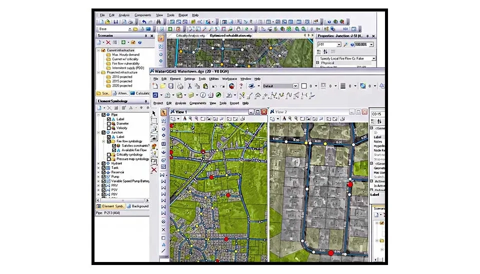
WaterGEMS is a commercial software package developed by Bentley Systems, WaterGEMS provides a comprehensive suite of tools for designing, analyzing, and optimizing water distribution systems (Bentley).  

WaterGEMS was developed by Bentley Systems, USA, for building hydraulic models of water distribution systems. WaterGEMS offers high interoperability with features for building geospatial models, optimizing design, and asset management. WaterGEMS provides an easy-to-use environment for engineers to analyze, design, and optimize water distribution systems (N.R. Kadhim et al., 2021).

1. WaterGEMS Software

A water distribution network offers consumers healthy sources of water using hydraulic components, such as pipes, valves, pumps, and tanks. WaterGEMS is hydraulic modeling software used to analyze and design water distribution networks. WaterGEMS is a hydraulic modeling for water distribution systems with advanced cooperation, geospatial model building, optimization, and management capabilities. WaterGEMS software has a comprehensive feature set compared to other software, including (Abdulsamad, A. A., Abdulrazzaq, K.A. 2023; Bentley):

Hydraulic Modeling: WaterGEMS offers advanced hydraulic modeling capabilities, including steady-state and transient simulations to assess network performance under various conditions.  

Water Quality Modeling: It can simulate water quality parameters, such as chlorine residual, temperature, and pH, helping to ensure safe drinking water.  

Pump Station Modeling: The software allows for detailed modeling of pump stations, including pump curves, energy consumption, and control strategies.  

Reservoir Modeling: WaterGEMS can model various types of reservoirs, including elevated tanks, ground storage tanks, and surface water sources.  

Network Optimization: The software provides tools for optimizing pipe diameters, pump schedules, and reservoir operations to minimize costs and improve efficiency.

Hydraulic Analysis: WaterGEMS can perform detailed hydraulic analysis, including pressure head calculations, flow velocity calculations, and pipe network optimization.  

Water Quality Analysis: The software can simulate water quality parameters, such as chlorine residual and temperature, to assess the impact of various factors on water quality.  

Transient Analysis: WaterGEMS can simulate transient conditions, such as pump starts and stops, to analyze the dynamic behavior of the network.

Key Features of Modern Water Distribution Design Software:

Hydraulic Modeling: Simulating network water flow under various conditions, including steady-state and transient analysis.  

Water Quality Modeling: Analyzing water quality parameters, such as chlorine residual and pressure.  

Optimization Tools: Identifying optimal design solutions, such as pipe sizing and pump scheduling.  

GIS Integration: Integrating geographic information systems (GIS) to visualize and analyze spatial data.

Uncertainty Analysis: Assessing the impact of uncertainties in input parameters on model results.

Why do engineers prefer WaterGEMS software over other software existing?

WaterGEMS provides many benefits beyond platform versatility. Here are four highlights:

1. It offers a friendly and intuitive interface, promoting a quick learning curve.

2. WaterGEMS supports multiple steady-state and extended-period simulation scenarios, which makes WaterGEMS ideal for master planning. It also uses system growth analysis, new land use mapping, and operation strategy modeling to plan confidently.

3. WaterGEMS automates pressure zone identification and analysis. Users can quickly define and visualize pressure zones to identify each zone's expected flow and maximum, and minimum values for pressure and hydraulic grade.

4. Water quality analysis is versatile and simple to configure. You can create simple water quality simulations for constituent (e.g., chlorine) concentration, water age, and source tracing or use advanced tools for multispecies analysis (MSX) and water quality batch runs.

WaterGEMS allows you to seamlessly integrate with CAD, GIS, and standalone platforms. This flexibility enables you to leverage the strengths of each platform to optimize your modeling processes, including:

• Windows for ease of use, accessibility, and performance.

• ArcGIS for GIS integration, thematic mapping, and publishing.

• AutoCAD for CAD layout and drafting.

2. Case Study: Henrietta

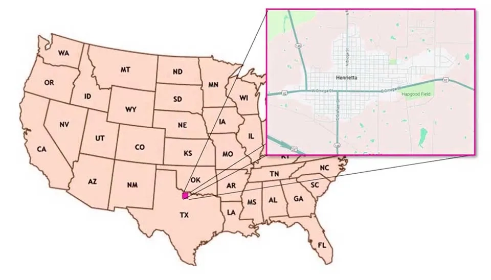
We selected Henrietta City for this project. Henrietta is one of the oldest settled towns in north central Texas. It sits at the crossroads of U.S. Highway 287, U.S. Highway 82, State Highway 148, and Farm to Market Road 1197 in north central Clay County., with coordinates 33°48′53″N 98°11′33″W. Henrietta’s population will be 3300 people in 2024. According to the United States Census Bureau, Henrietta has a total area of 5.2 square miles (13.5 km2), of which 5.1 square miles (13.2 km2) is land and 0.1 square miles (0.3 km2), or 1.96%, is water (world population review). It is situated 915 feet (279 m) above sea level. The below figure illustrates the location of Henrietta in the state of Texas. The climate in this area is characterized by hot, humid summers and generally mild to cool winters. According to the Köppen Climate Classification system, Henrietta has a humid subtropical climate.

3. Design of Water Distribution Network Using WaterGEMS

Water networks are an essential part of urban infrastructure, and major investments are associated with providing the required capacity (Cunha and Marques, 2020).

WaterGEMS software is developed for the design and analysis of water supply networks or the expansion of existing networks. The software provides the required standard and economical platform for the design, analysis, and troubleshooting of new and existing supply networks with accuracy and minimum time duration. WaterGEMS software gives optimal solutions for all types of networks. The property of WaterGEMS software is that it can be used to accurately simulate a network before it has been built or modified. The simulation of network problems can be easily identified and removed so that expensive errors can be avoided (S. Pathan and Kahalekar, 2018). However, much of this software is complex and difficult to apply techniques in real networks in developing countries, which have fewer skilled manpower. Recently, it has been easier to model and optimize theories with the help of WaterGEMS (Water Geospatial Engineering Modeling System) software. This software is suitable for hydraulic models to optimize the WDS worldwide using the Darwin Designer and Darwin Scheduler tools based on the Genetic Algorithm (GA) (Switnicka et al., 2017).

3.1. Basic Requirements for Design 

The essential requirements to design a water distribution network  include

1. Hydrological information: the amount of participation, evaporation and transpiration, river flow, water table resources

2. Population information: the population now and projected population in the future, patterns of water consumption, and population growth

3. Preparation of a map of the study area

4. Topography information: the topography of the area, the slope of the land, and geology information

5. Available the water distribution network: pipes, reservoirs, pumps, and other available types of equipment

 3.1.1. Population and its Prediction Methods

Initially, we gathered information about the current population of the study area. After that, it is necessary to use the below formula to calculate the population in the future. Three methodologies are commonly employed for forecasting future population trends. Consequentially, these techniques involve 

1) Arithmetical Increase Method 

2) Geometrical Increase Method 

3) Incremental Increase Method

 (T. Mavi and D.R. Vaidya, 2018; Mekonnen YA, 2018). 

3.1.1.1. Arithmetical Increase Method

The arithmetic increase method assumes that the rate of population change remains constant over time. It is typically applied to older and larger cities with no significant industrial growth and where development has reached saturation or maximum capacity. This method tends to yield lower projections for rapidly growing cities. Below, the calculation process and components of the formula are explained (T. Mavi and D.R. Vaidya, 2018; Mekonnen YA, 2018).

Pn = (P0 + n.x)

Where

p0 = current population;

Pn = prospective population after n decades.

x = average increases in population per decade.

n = decades

3.1.1.2. Geometrical Increase Method

The percentage increase method assumes that the percentage increase in population remains constant from decade to decade. This method is particularly suitable for young and rapidly expanding cities, as it accounts for exponential growth trends. (Mavi and Vaidya, 2018;  Dinh et al., 2022;  Mekonnen YA, 2018). The formula for this method is as follows:

Pn = P0 [ 1 + ( r/100 ) ]^n

p0 = current population;

Pn = prospective population after n decades.

r = geometric mean percentage increase.

n = decades

Pn = 3300[ 1 + ( 0.1/100 ) ]^10

3.1.1.3. Incremental Increase Method

The population change rate over time is taken to be constant in the Incremental Increase method. Applicable to large, historic cities that have reached their maximum development or saturation and have not experienced industrial growth (Mavi and Vaidya, 2018; Biaknghinglovi et al., 2018). For cities that are expanding quickly, this approach produces less accurate results.

Pn = (Po + nx̄) + ((n(n+1))/2)* ȳ,

where,

P0 = last known population,

Pn = population (predicted) after 'n' number of decades,

n = number of decades between Po and Pn,

x̄ = mean or average of increase in population and,

ȳ = algebraic mean of incremental increase (an increase) of population

Because the world’s population is increasing, the third method is the best for predicting the future population. This method is a modification of the arithmetical increase method, and it is suitable for an average-size town under normal conditions where the growth rate is found to be in increasing order. When using this approach, the future population is calculated, taking into account the increase in increment. The incremental increase is calculated for every decade from the previous population, and the average value is added to the current population along with the average rate of increase. Based on these projections, the population of Henrietta is estimated to be approximately 5,800 in 2024. To forecast the population of the city of Henrietta, the population must be between three and five decades old. To avoid mistakes, the calculation should be completed in Excel. The results table should then be copied from the Excel or Google sheets program and placed here.

You can click here to access Henrietta Population Prediction base on Incremental Increase Method.

Table 1.The population of Henrietta for 5 decades recent

According to the CPHEEO standard, a thirty-year prediction period is taken into account. Using the incremental increase method, we can forecast the population for 2034, 2044, and 2054 based on the information in the table.

Population in 2034 

P[2034] = {P[2024] + (nx̄)} + ((n(n+1))/2)* ȳ

P2034 = {3300+ (100×1)} + {(1×(1+1))/2} × 50= 3450

2044

P2044 = {3300+ (100×2)} + {(2×(2+1))/2} × 50= 3650

and 2054

  P2054 = {3300+ (100×3)} + {(3×(3+1))/2} × 50= 3900

The life span of each part of the urban water supply system should be estimated; rough estimations are given here. This estimation is also important to evaluate the maintenance cost of the system and amortization, thus allowing planning of further development stages. The table below shows any part of the urban water supply system (Water Demand, 2014).

Table 2.The lifespan of each part of the Urban water supply system 

 3.1.2. Calculation of The Water Requirement in The Study Area

Overall, for calculating the demand for a city, several factors must be considered, such as population demand, minor losses, fire demand, and unaccounted-for water (J. C. Agunwamba et al., 2018). The total demand for designing the water distribution network involves some items that include the following:

1. The per capita demand: This item is the average daily demand by residents for drinking, cooking, bathing, washing cloth, washing utensils, washing houses, gardens, and flushing; this is variable for any country (Code of Basic Requirements for Water Supply, Drainage, and Sanitation). However, the per capita Demand is different in The USA (Public Supply and Domestic Water Use in the United States, 2015).

2. The daily demand: This item is the amount of demand on base gallons per second for the city population.

3. The fire demand: The amount of water required to fight a fire depends on the building's density and height. However, the amount of fire demand is often estimated as a percentage of the total daily demand, typically ranging from 5% to 10% (Adeniran & Oyelowo, 2013; J. C. Agunwamba et al., 2018),

4. The minor losses: Water minor loss in the distribution network occurs due to friction in pipes, fittings, and valves. It is estimated as a percentage of the total daily demand, typically around 5% (U.Terlumun and E.Robert, 2019; J. C. Agunwamba et al., 2018).

5. Unaccounted-for Water (UFW): The water that is lost due to leakage or theft, which is known as Unaccounted-for Water (UFW) is the difference between the volume of water supplied to a distribution network and the volume that is legitimately consumed and billed. The American Water Works Association (AWWA) recommends a benchmark of 10% for UFW, with a focus on reducing losses between 10% and 25%, while losses over 25% are considered problematic. UFW is expressed as a percentage of the water delivered and includes both physical losses (like overflow and leaks) and non-physical or commercial losses. Reducing UFW can enhance the availability of drinking water. (U.Terlumun and E.Robert, 2019; Z.Y. Ahmed, 2024). While the main references recommend using a range between 10 and 25%, most engineers choose around 15% based on their experiences. Ultimately, the employer gives an opinion on the appropriate amount of unaccounted water (UFW), and they may select UFW more than 15% or less than 15% because they are more familiar with the study area than designers.

6. Total Demand: It includes the sum of items 1 to 5 according to the design for the next 30 years (2024 years). Therefore, a demand of 5.43 Gal/s was selected for a design using WaterGEMS software. 

The table below illustrates the estimated demand for Henrietta in 2024, 2034, and 2024. To avoid mistakes, the calculation should be completed in Excels or Google Sheets.

You can click here to download Calculation of The Demand for Henrietta case study.

Table 3. Analysis of Demands for  the City of Henrietta

The table provides an analysis of water demands for the City of Henrietta, Texas, from 2034 to 2054, highlighting the increasing demand due to population growth. The population rises steadily from 3,450 in 2034 to 3,900 in 2054, directly impacting water usage. The per capita demand remains constant at 92.5 gallons per day, indicating stable individual water consumption over time. As a result, the daily demand increases from 3.69 gallons per second in 2034 to 4.17 gallons per second in 2054. Fire demand, calculated as 10% of daily demand, rises proportionally, starting at 0.37 gallons per second in 2034 and reaching 0.42 gallons per second in 2054. Minor losses, estimated at 5% of daily demand, also increase slightly, from 0.18 gallons per second to 0.21 gallons per second over the same period. Unaccounted-for water (UFW), representing 15% of total demand, grows from 0.55 gallons per second in 2034 to 0.63 gallons per second in 2054. Consequently, the total water demand for the city increases from 4.80 gallons per second in 2034 to 5.43 gallons per second in 2054, emphasizing the need for enhanced water distribution planning to meet future demands.

3.1.2.1. The Daily and Hourly Peak Factors 

The daily peak factor represents the ratio of the maximum daily demand to the average daily demand. It accounts for the variation in water demand throughout the year., which is influenced by factors such as seasonal changes, holidays, and economic activities. Moreover, the hourly peak factor represents the ratio of the maximum hourly demand to the average hourly demand on the day of maximum demand. It accounts for variations in water demand within a day, such as peak hour usage in the morning and evening.

3.1.2.1.1. The daily peak factor (C1)

The daily peak (C1) is determined according to the criteria measured at the time of the project study, people's water consumption habits, and measurements taken in similar cities, which ultimately show this coefficient according to the climate of the region. Then, according to the average per capita consumption and the coefficient (C1), the maximum daily consumption is determined (AWWA; Cabral et al. 2016). This factor always ranges between 1 and 2. When the area's weather is colder, people consume less water; thus, this factor is closer to 1. Additionally, when the area's weather becomes hotter, it approaches 2 because people need to consume more water. As a consequence, this factor directly results in increasing demand. For example, a city might experience a hot month in summer throughout the year, and this month can be used to determine the daily factor for designing (water and wastewater engineering). According to the weather conditions in Henrietta, it is a semi-arid climate, and the appropriate daily peak factor (C1) is approximately 1.8 (PWD; B Syahputra et al., 2022; Water Demand Analysis). This choice for (C1=1.8) is an offer that, finally, the designer and employer decide the amount of the daily factor for design.

3.1.2.1.2. The Hourly Peak Factor (C2)

One of the main factors in determining the amount of hourly factor is the population (T. BERGEL et al. 2018). In urban areas, the per capita water consumption is typically higher. Instead, the maximum hourly coefficient tends to be lower. Conversely, in rural areas, the per capita water consumption is generally lower. Instead, the maximum hourly coefficient is higher. This factor prevents excessive pressure on the network during peak times, such as mornings and evenings when consumers need to use water. Therefore, the value of the hourly factor is determined from the table below.

Table 4.The peak factor for water demand

Therefore, the hourly peak factor (C2) is set at 3 for Henrietta City.

According to the daily and hourly peak factors, the demand can be calculated:

The maximum demand ⇒ Initial demand*C1*C2 ⇒5.43*1.8*3 = 29.32 ⇒ 

Therefore; the maximum demand: Q max=29.32 Gal/s.

3.1.3. Location Map And Elevation Points of The Study Area

WaterGEMS software is a user-friendly software that can link with ArcGIS software or any software like Global Mapper software that can create shapefiles for importing to WaterGEMS software as pipes and nodes; also, the AutoCAD software. Also, the AutoCAD software creates DXF and DWG files. Next, we will familiarize you with ArcGIS, Global Mapping, and Autocad software products. Learn how to develop pipes in Shapefile or DXF AND DWG format. We have discussed the design of the pipe network analysis using WaterGEMS software for Henrietta. The Henrietta town master considers it as a reference for designing the network.

3.1.3.1. Creating Shapefile Format with ArcGIS Software

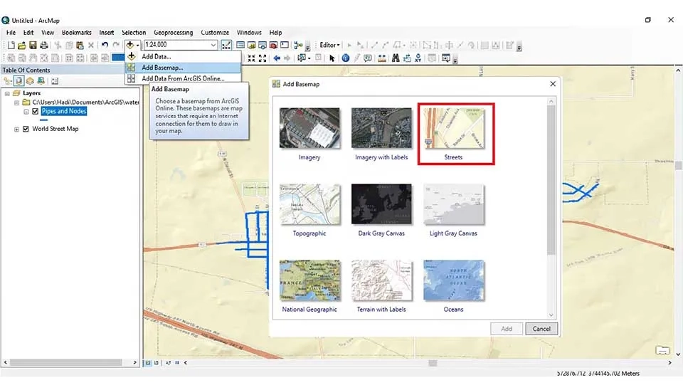
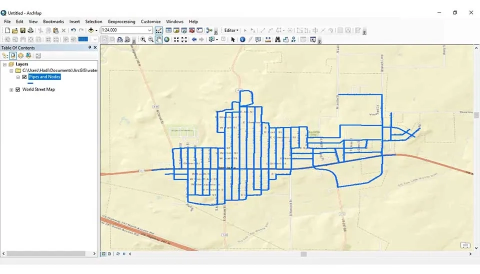
This method involves directly drawing pipes in ArcGIS using the Basemap in process, which provides information including geographic details, such as roads, cities, countries, waters, and mountains, from the target city information. This allows for creating pipes and nodes specifically for the city's layout. The resulting format is a Shapefile, which can be imported to design the water distribution network.

3.1.3.2. Creating Shapefile Format with Global Mapper Software

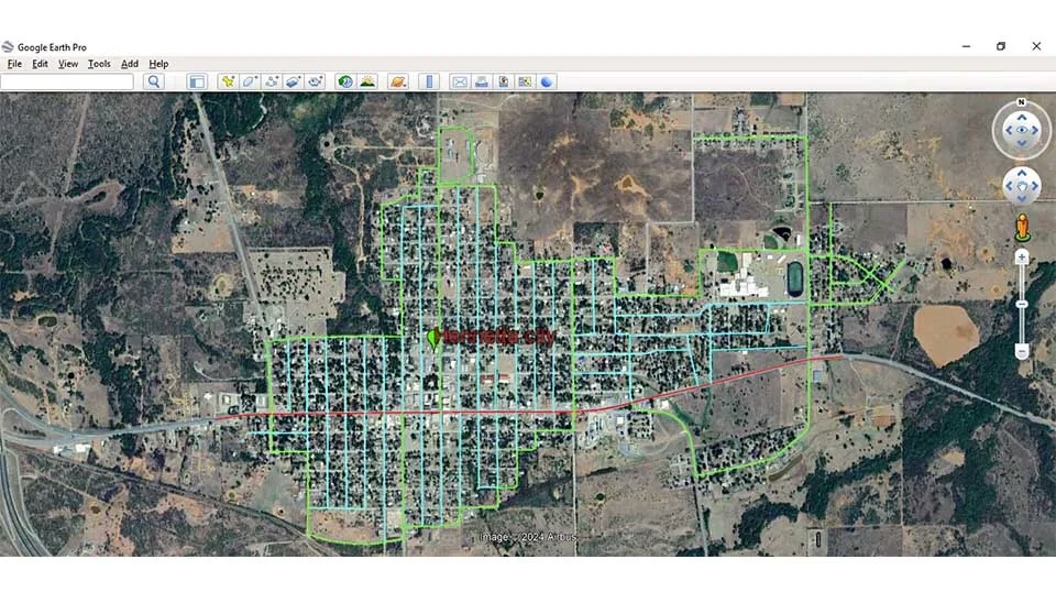
To create a shapefile format for the city’s water distribution system, the process begins with Global Earth. In this software, the pipe network for the city is manually drawn and saved in KMZ format. While KMZ is a widely used format, it is not directly compatible with GIS-based software like WaterGEMS, which requires shapefiles for accurate integration. To address this, the KMZ file is imported into Google Maps or similar GIS tools for conversion. Using specialized tools or software (e.g., QGIS, ArcGIS, or online KMZ are used to shapefile converters). The KMZ file is transformed into the shapefile (.shp) format. The resulting shapefile contains georeferenced data essential for importing into WaterGEMS or other hydraulic modeling software. This process ensures seamless integration of geographical and network data, enabling detailed analysis and simulation of the water distribution system.

The figure illustrates the process of drawing a water distribution network using Google Earth Pro. The map shows a detailed layout of pipes designed for the city, which is represented with green lines. This process involves manually plotting the pipe network over the city’s satellite imagery, ensuring an accurate representation of the geographical and infrastructural layout. 

Once the pipe network is completed in Google Earth, the data is saved in KMZ format. This format is later converted into Shapefile (.shp) format for further analysis and hydraulic modeling in tools like WaterGEMS. This step is essential for integrating real-world geographic data into the simulation process, ensuring precise modeling of the water distribution system for planning and optimization.

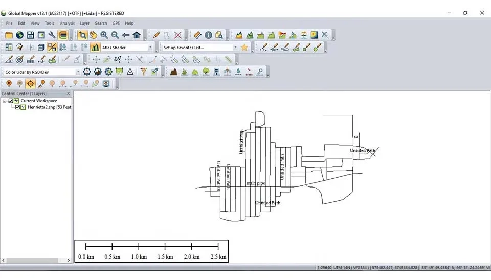
The figure demonstrates the next step in the process, where the KMZ file created in Google Earth is imported into GIS software, such as Google Maps or QGIS, for conversion into a Shapefile (.shp) format. The imported network is represented as a simplified schematic of the pipe layout for the City of Henrietta, preserving its spatial accuracy and structure.

3.1.3.3. Creating DXF and DWG Formats with AutoCAD Software

It will use DXF and DWG files in two different methods to create a pipe in the WaterGEMS software. The first method is identical to the previous methods, where the DXF and DWG files are imported from the ModelBuilder section of WaterGEMS to create pipes. The second way will opt for a map as the background of the area of the case study to draw pipes in the waterGEMS. Also, the output of any of the above methods can be obtained in the formats DXF and DWG. Each of these two methods will be explained in the following tutorial.

4. Simulation and Design by WaterGEMS Software

In this stage, we will provide users with a step-by-step guide, starting from the creation of a new project to obtaining the final outputs. Each step will be explained in detail, ensuring clarity and ease of understanding for both beginners and experienced users. The process will cover essential tasks such as setting up the model, defining system components, running simulations, analyzing results, and generating meaningful outputs. By following these instructions, users will gain a comprehensive understanding of how to effectively simulate and design water distribution systems using WaterGEMS.

4.1. Creating a New Project

The first step involves creating a new project in WaterGEMS. This serves as the foundation where you can perform all the necessary tasks for modeling and analyzing the water distribution system. From setting units and importing data to running simulations and optimizing the design. The new project acts as the workspace for managing every aspect of the modeling process.

To create a new project, the following steps have to be followed: 

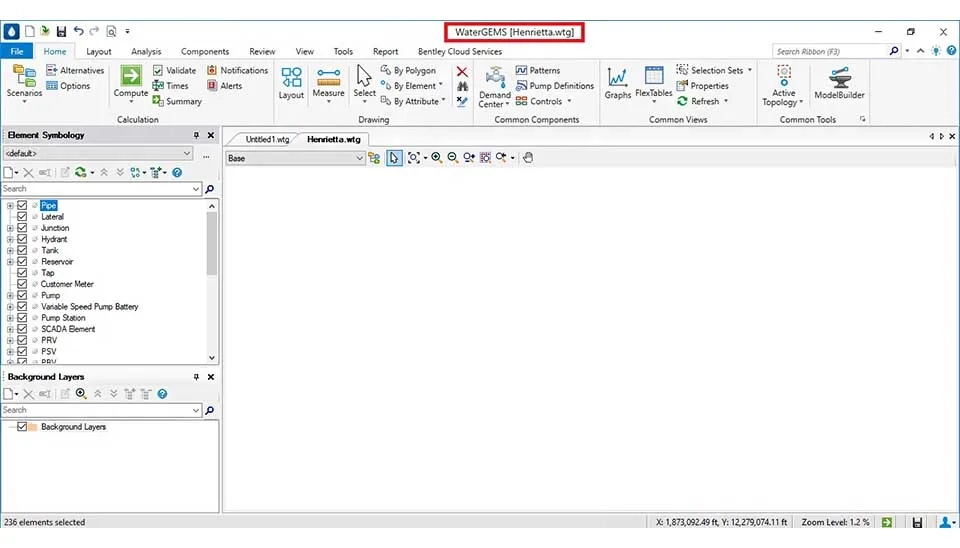
1. Navigate to the top menu and select File > New, or click the New Project icon available on the General Toolbar. This will initiate the creation of a new project.

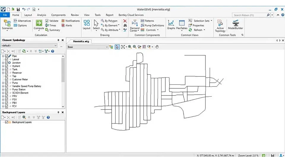
2. A new unnamed project is created, displaying all the default options and tools necessary for designing and analyzing water distribution networks, which is shown in the figure below.

3. Whenever WaterGEMS is launched, a new project is automatically created, allowing users to begin their work immediately without the need for manual initialization.

Now that the new project has been created, it is essential to configure the units and scale settings to ensure accurate modeling and analysis. These settings define the measurement units for parameters, such as flow, pressure, and pipe lengths, as well as the spatial scale for the network. Proper configuration is crucial for consistency and precision in simulations. The following section will guide you through the process of setting up units and scale in WaterGEMS.

4.2. Setting Units and Scale 

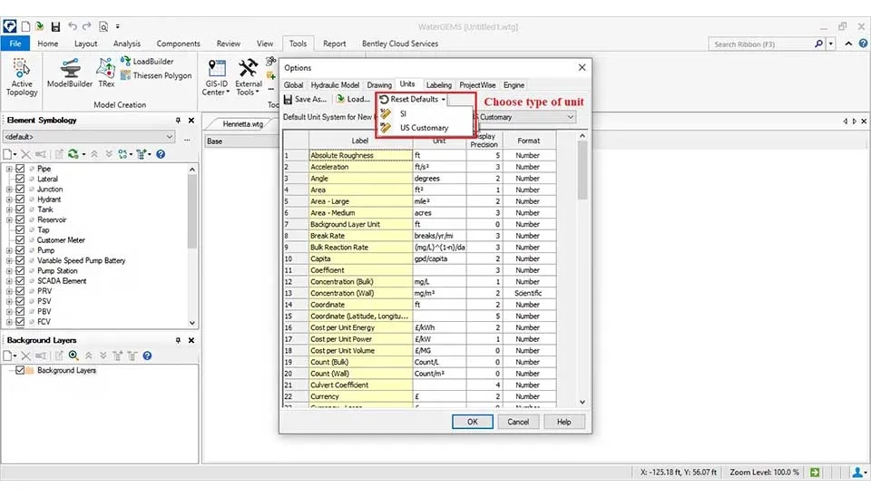
At this stage, the setting units and scale can be configured using the following paths:

1. Select the Tools option in the menu bar and click on OPTIONS. 

2.  A DIALOGUE BOX appears with different options. 

3. Select UNITS, click on the SI unit and change the units for each parameter.

4.3. Importing Pipes and Nodes in WaterGEMS Software

The ModelBuilder item, including pipes and nods, is used in the menu bar to transfer Shapefile.

To access ModelBuilder, click the Tools menu and select the ModelBuilder command or click the ModelBuilder button.

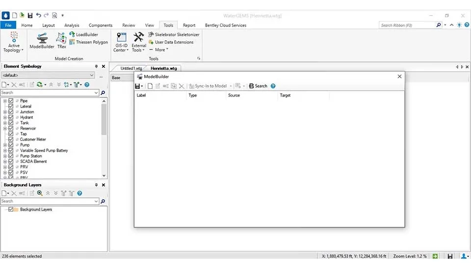
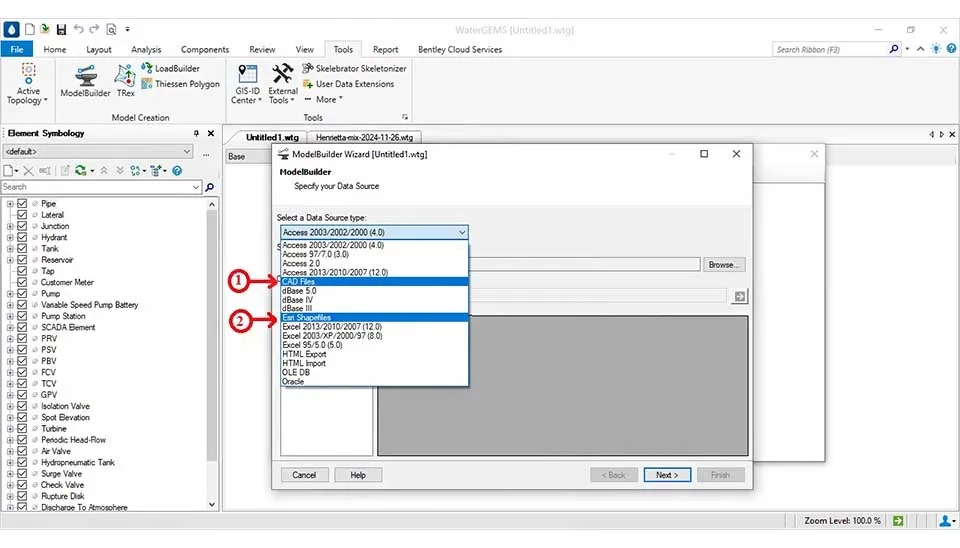
In this step, click on New, then open the ModelBuilder Wizard from the drop-down menu. Select a Data Source type and choose the kind of file or reference software, which opts for Esri Shapefiles or DXF and DWG files. The figure below indicates that we will use number one for DXF and DWG files, and number two for the Esri Shapefiles file. You can select and preview the desired database tables. Therefore, click ‘Next’ to proceed to the next step.

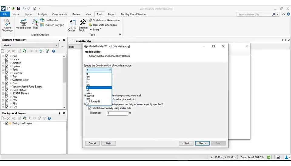
Next, the unit of your data source is set (drop-down list); additionally, check boxes for  “Create nods if none are found at the point endpoint” and “Establish connectivity using spatial data” to be chosen.

Note: When working with shapefile, the unit is automatically set to ‘’m’’. However, the unit must be set with “m” when working with WaterGEMS. Otherwise, this can confuse if your shape working units are "ft.".

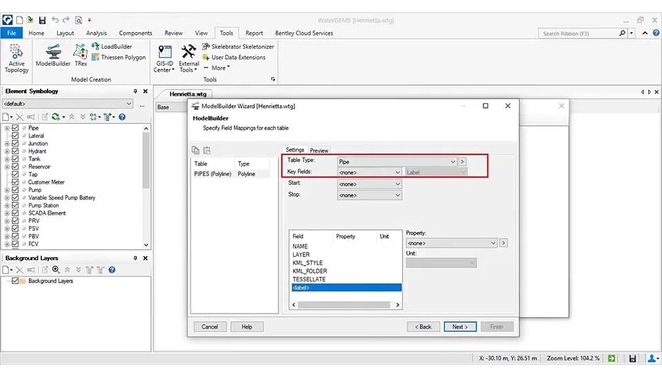
Like the figure below, the pipe is chosen as the ‘table type’. Additionally, the label needs to opt in ‘Key Fields’. Therefore, it is clicked ‘Next’ to proceed to the next step.

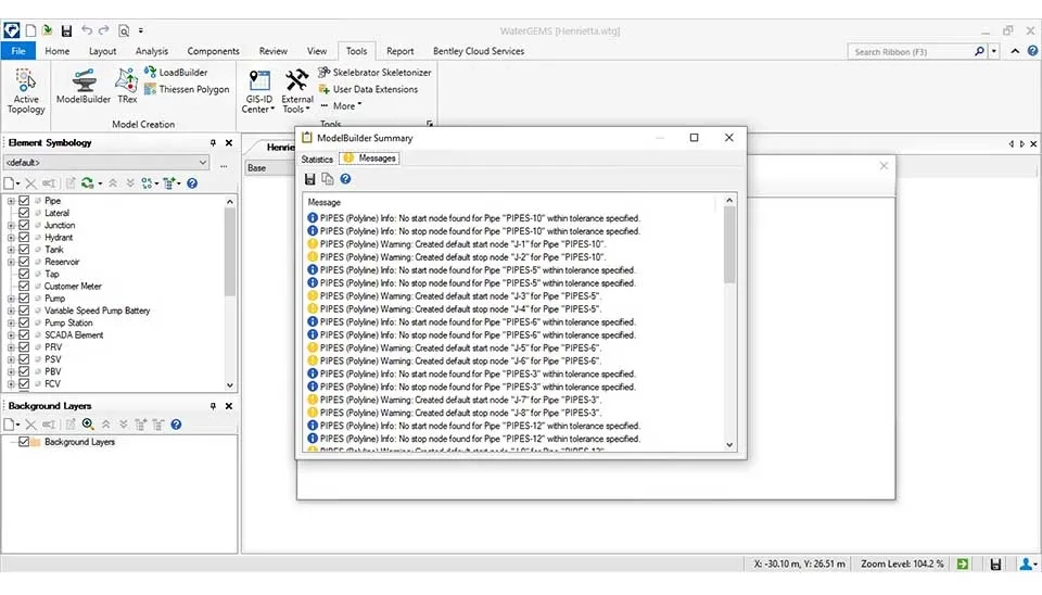
Finally, it is clicked ‘Finish’ to proceed to the end step. If the software shows you the below figure messages with yellow and blue colors, it means all steps are accurate; on the contrary, it illustrates a message with red color. Indeed, one of the ways is wrong. Consequently, it is necessary to fix that particular case.

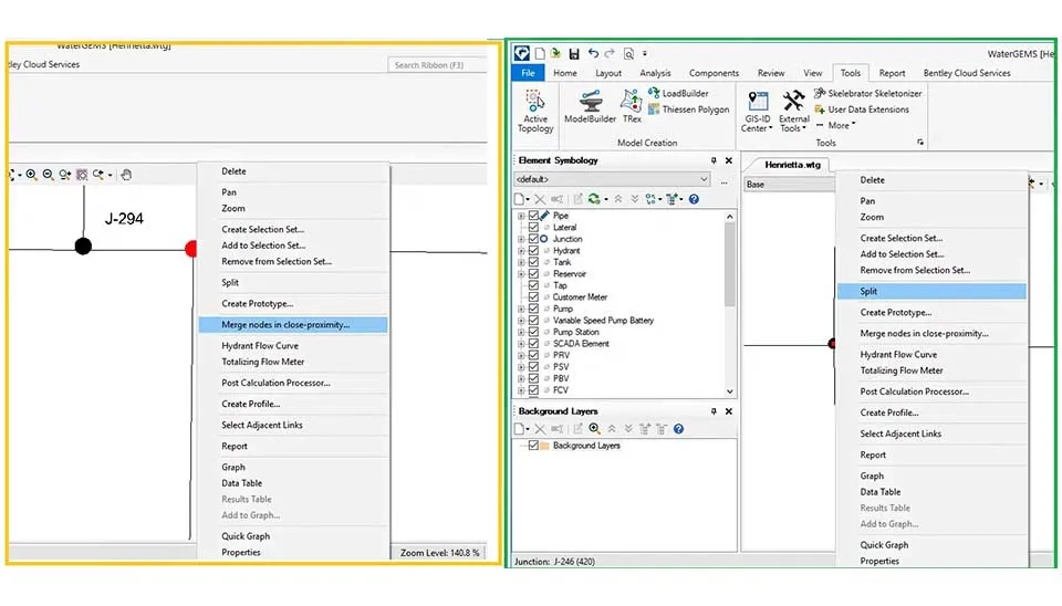
Note: After completing all the steps, it is essential to double-click on the main page of WaterGEMS so that the pipes and nodes are shown. Additionally, there may be some nodes and pipes that are not connected. Therefore, it is crucial to address these issues manually. This means that pipes and nodes are connected using the 'Split' method, while nodes are linked through the 'Merge nodes nearby' technique.

Another approach is to utilize a map from the case study area as a background in WaterGEMS software. This method allows for the direct creation of pipes and nodes.

The following sections will explain how to draw pipes and nodes directly within the WaterGEMS software.

First, a map of the case study area must be provided in the *.TIFF file format. This TIFF file will be created from a photograph of the case study area.

There are several methods available for generating a TIFF file.

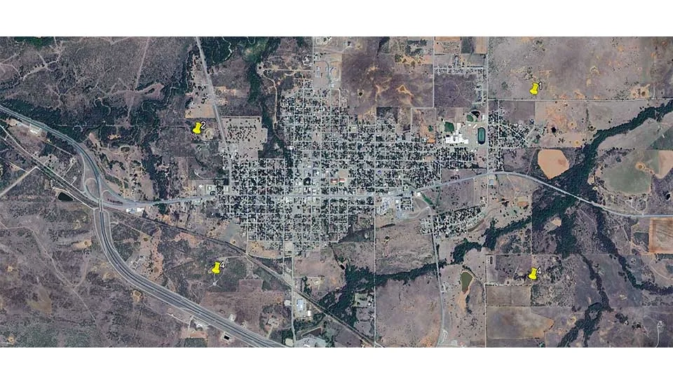
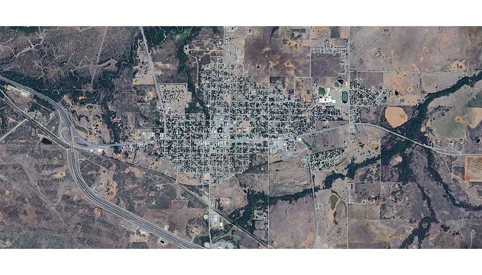
Initially, the image is acquired from the case study area using Google Earth Software. After obtaining the image, it must be georeferenced with Global Mapper Software. To do this, three or four coordinates from the case study area need to be sourced from Google Earth Software. When selecting the points, they should be chosen following the guidelines illustrated in the figure below,  The points should be chosen from four distinct zones.

The image needs to be free of elements like those shown in the figure below for georeferencing.

Next, we will use the Global Mapper software to georeference the image. The steps for georeferencing with Global Mapper Software include:

1.  To import the image into the software, click on 'Open Data Files.'

2. Before opening the image in Global Mapper software, a dialog box titled 'Select Position to Use for Layer' appears. This box contains three options, and you should choose the first one, 'Manually Rectify Image.'

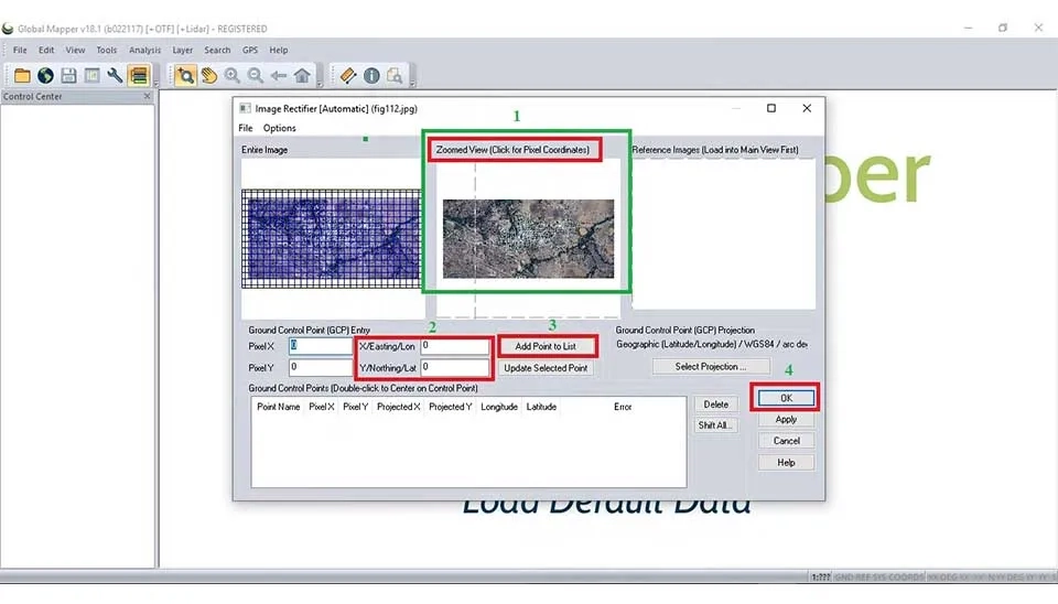
After selecting this option, you will need to specify the exact coordinates of the location in the 'Zoomed view (click for pixel coordinate)'.

1.  It will be used to import any coordinate throughout boxes X/Easting/Lon and Y/Northing/Lat; after that, click on the ‘’Add Point to List’’ for any coordinate. Finally, all coordinates will be imported; click on ‘’OK’’. Therefore, we have completed all the necessary steps to create a TIFF file. Now, it can import the TIFF file in WaterGEMS Software.

Adding TIFF File to WaterGEMS Software

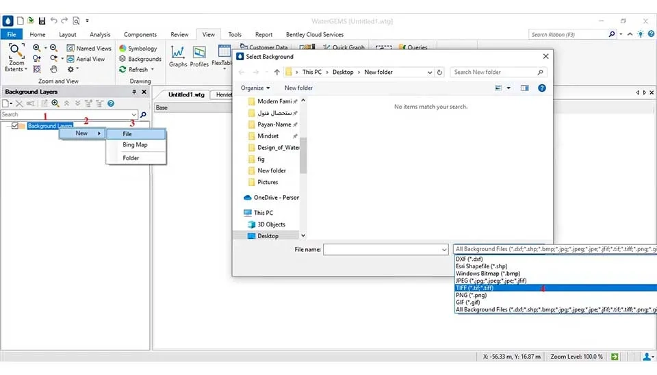
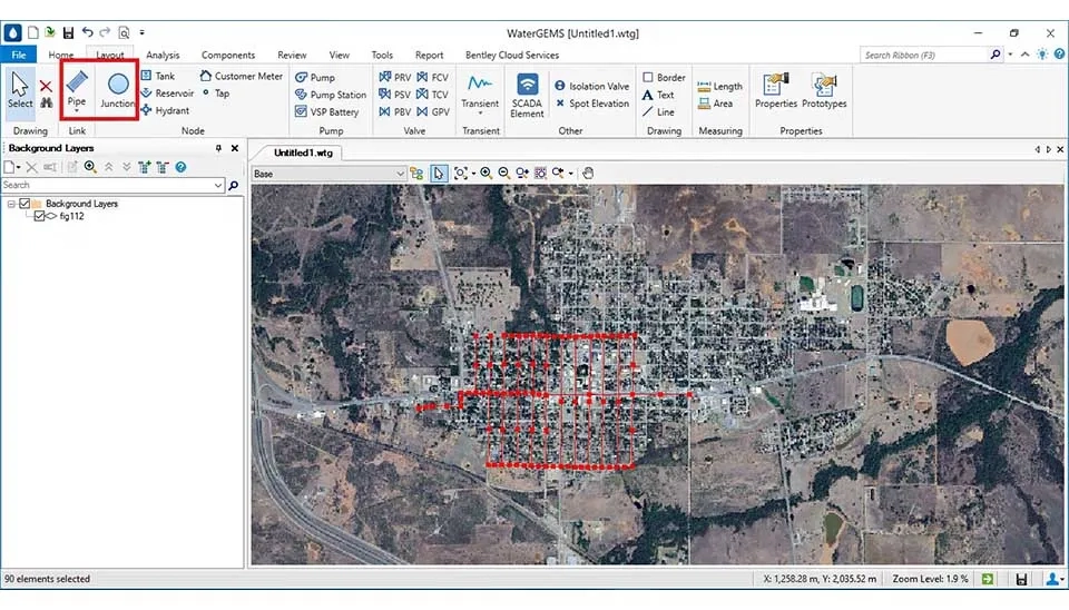
First, you need to add 'Background Layers' to the WaterGEMS software interface. Next, right-click on 'Background Layers' and select 'New' → 'File.' This will open a window where you can choose the 'TIFF (*.tif; *.tiff)' format. Lastly, select the desired TIFF file from your computer.

Before selecting the TIFF file, it is necessary to export the X and Y coordinates from the TIFF in the GIS software. This step is essential before importing the TIFF file into the WaterGEMS software. Finally, the coordinates X and Y, along with the TIFF files, will be imported into the WaterGEMS software.

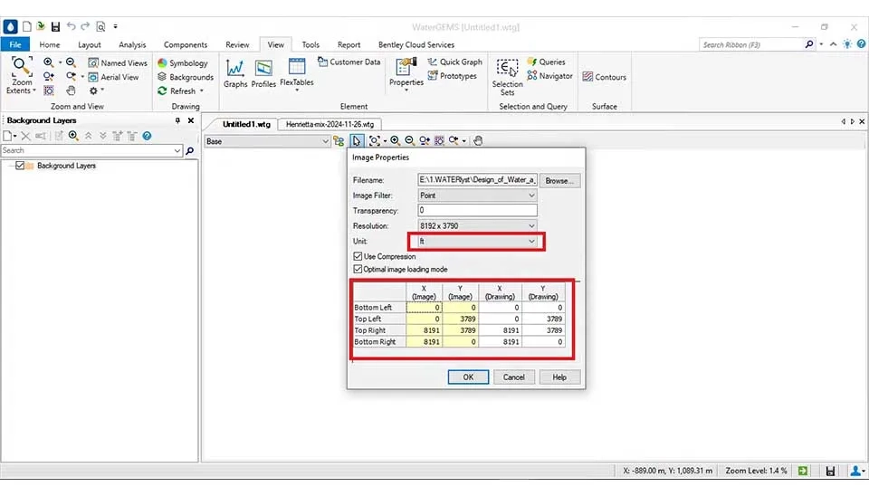
As a result, pipes and junctions will be used to create pipes and nodes based on the TIFF file in the layout section of the WaterGEMS software. The figure below illustrates these steps.

4.4. Importing Elevation Data of Nodes

The TRex Wizard automatically assigns NodeS elevations using data from a Digital Elevation Model (DEM) or a Digital Terrain Model (DTM). Valid elevation data sources include:

• Vector files such as DXF and SHAPefiles

• LandXML files

• InRoads .dtm (Microstation platform only)

• Geopak .tin (32-bit version only)

• Bentley MX .fil

• Bentley .dgn (Microstation platform only)

In this step, the nodes need to have elevation data that is mapped to the study area or a file raster of the study area is required. 

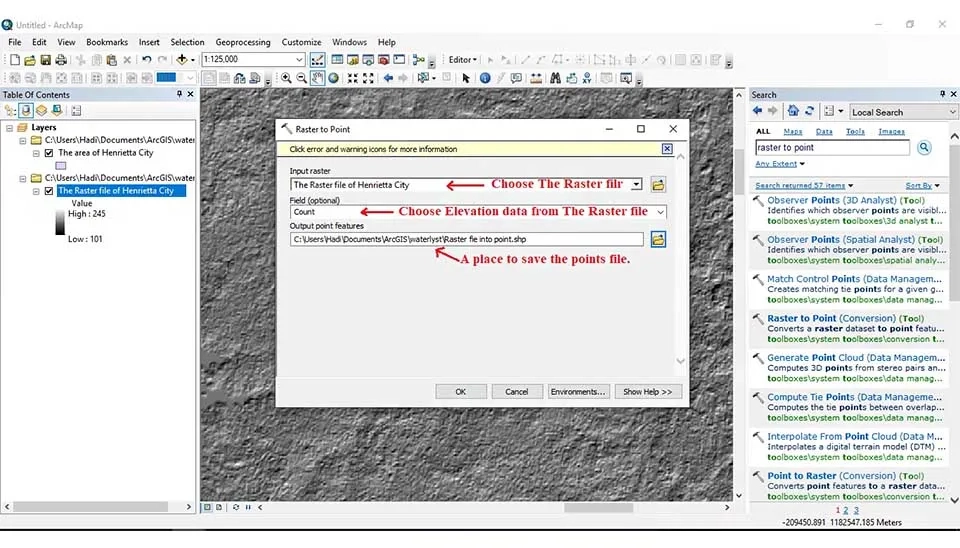
The file Raster is used in this project for the elevation data of nodes. The USGS Earth Explorer is used to download Raster files. Additionally, some satellites, such as Open Topography, Sentinel Satellite Data, and EarthExplorer sites, are used to download Raster files. Therefore, this project uses the raster file, including the digital elevation model (DEM) that must change the raster file into points by ArcGIS software. The file Raster is used in this project for the elevation data of nodes. The USGS Earth Explorer is used to download Raster files. Also, some satellites, such as Open Topography, Sentinel Satellite Data, and EarthExplorer sites, are used to download Raster files. This project will use the Raster file, including a digital elevation model that must convert the Raster file to  Points by ArcGIS software. Refer to this tutorial file to learn how to download a raster file from reputable sites also convert it into elevation points in GIS software for use in WaterGEMS software.

4.5. Import the Elevation Data to WaterGEMS Software

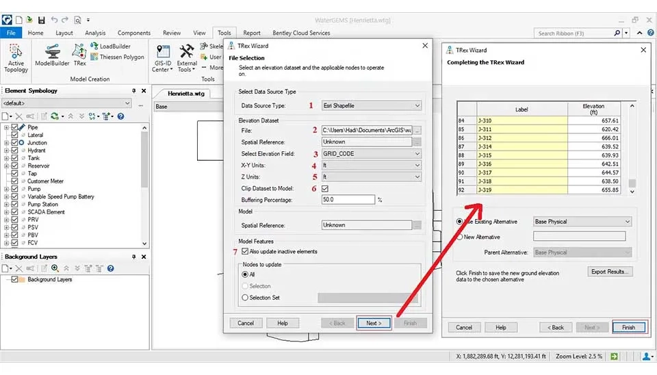
Select the Tools option in the menu bar and click on TRex. The steps of this method include:

Firstly, you need to choose the types of data sources mentioned earlier. However, this project will utilize the Shapefile format.

Secondly, select the file containing the Elevation Data on your computer

Next, select the elevation field.

Then, choose the type of units for your project.

Note: We need to check the boxes. Steps 6 and 7 are illustrated in the figure below.

After that, click the ‘Next’ button to proceed to the next level. Finally, all nodes will elevate to the next level. Additionally, click the ‘finish’ button to complete this step.

4.6. The Placement of The Reservoir in WaterGEMS Software

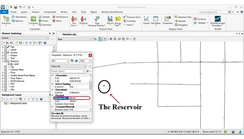
A reservoir serves as an example of a storage node. A storage node is considered a particular node category with a free water surface at the height of the water above sea level, which is called a hydraulic head. The elevation of the water surface indicates that the reservoir remains stable if water flows in or out during an extended period of simulation.

To apply for a reservoir, you need to follow the steps below:

1. The placement of the reservoir is better to be the highest of all the nodes. 

2.  Click the Tools menu, select the layout, and choose reservoir in the Node section.

3. A reservoir is created next to your mouse cursor, allowing you to select the location of the reservoir in the WaterGEMS software. 

4. Finally, click on the “Reservoir” to give it elevation.

4.7. Applying a Pump in WaterGEMS Software

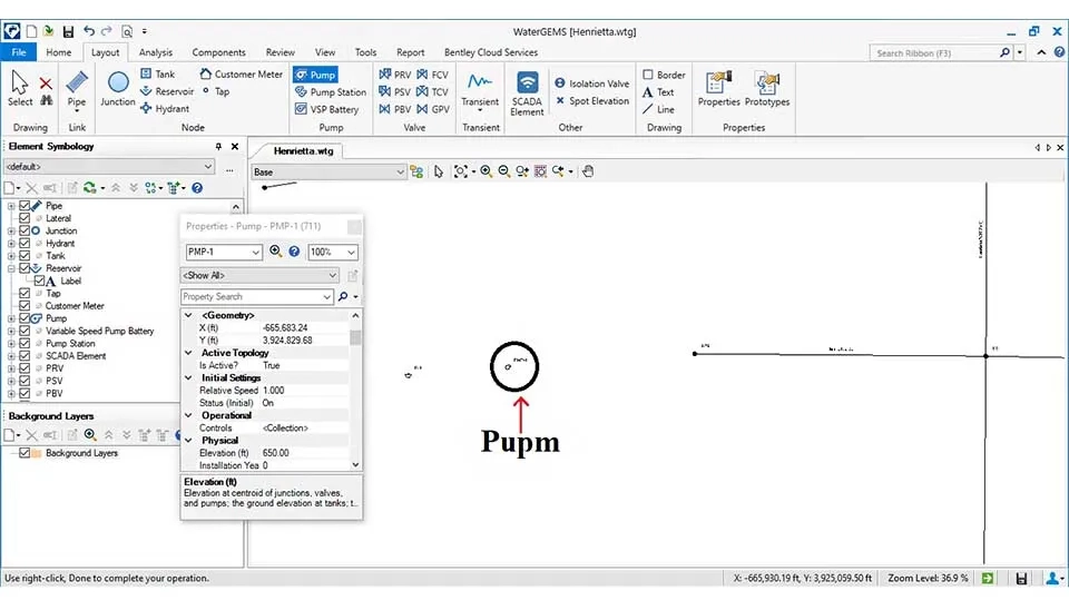
Pumps are used to impart energy to the water to either boost higher elevations or increase its pressure. Most pumps that are used in distribution systems are centrifugal. 

To define a pump, it is essential to follow the steps below:

1. The pump should be placed at a lower level or the same level as the reservoir. Click the Tools menu, select the "Layout,” and choose Pump in the “Pump” part.

2. A pump is created next to your mouse cursor, allowing you to select the location of the pumps in the WaterGEMS software. 

3. Finally, click on the “pump” to provide supplementary information. Include the elevation of the pump, its definition, and its functional characteristics.

Note: It is crucial to choose a pump as a reservation. In addition, according to the demand of the flow and pressure for the city, more than a single pump may be required for this design; therefore, it is necessary to use multiple pumps in the design process.

4.8. The Steps of Opting for The Pump

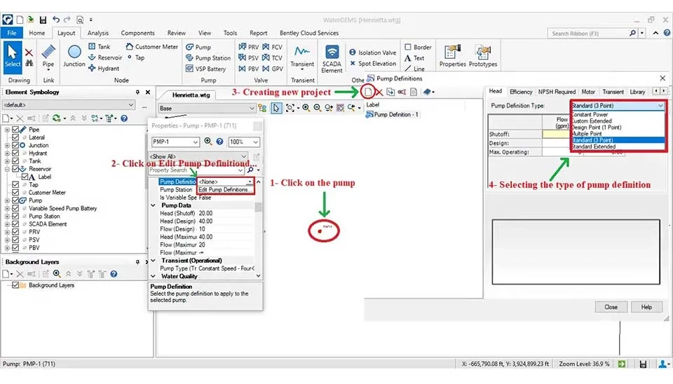
Initially, a single pump is used for the design if it is required to add more pumps. To select the pump, follow the method below:

1. Click on the pump on WaterGEMS Software, 

2. Select Components > Pump Definitions.

3. Click New to create a new pump definition.

4. For each pump definition, perform these steps: Select the type of pump definition in the Pump Definition Type menu. Type values for Pump Power, Shutoff, Design Point, Max Operating, and/or Max Extended as required. 

Additionally, we need to define efficiency and motor settings in the Efficiency and Motor tabs.

Selecting a type of centrifugal pump from the catalog requires two items: flow and pressure; therefore, the maximum demand is 54.86 gallons per second; a pump that is capable of providing the necessary energy to the water must be selected. However,  calculating pressure is different. Firstly, different elevations are required  in critical situations. The elevation difference in Henrietta is ∆H static = 47.9 ft  (maximum = 931.7 ft, minimum = 883.8 ft). Secondly, the pressure drop (Hf)  in the pipeline must be calculated as it is necessary for sizing the pipes. Otherwise, we cannot design it which means that we can determine the appropriate diameter of the pipe based on the demand and the optimal velocity. The minimum and maximum velocities for any pipe range between 0.3 and 3 m/s (Kassahun and Dargie, 2024). The formula for calculating the suitable pipe diameter is as follows:

Q = A*V

 ⇒ A = Q/V

Q = 23.92 gal/s ⇒ Q= 3.92 ft^3/s, 

V (optimal velocity) = 3.28 ft/s 

⇒ A= 1.2 ft^2, 

⇒ for calculating area, 

A = π*D^2/4, for calculating the Diameter, 

D = (4A/π)^0.5⇒ D= (4*1.2 / 3.14)^0.5

⇒ D = 1.24 ft m ⇒ D = 14.76 in 

Therefore, there are 14 and 16 inches diameters on the market. So, it is better to choose the larger diameter for proper hydraulic conditions  in design.  (D ≈ 16 in) 

To estimate Hf in a pipe, use the following formula:

h100ft = 0.2083*(100 / c)^1.852 * q^1.852 / d^4.8655                      

where

h100ft = friction head loss in feet of water per 100 feet of pipe (ft h20 /100 ft pipe)

c = Hazen-Williams roughness constant

q = volume flow (gal/min)

d = inside diameter of pipe (inches)

This is in the project: 

hf =?

Q = 29.32 (in gallons per second) ⇒1759.2 GPM

C = The choice depends on the type of pipe; this project uses STEEL pipe. 

Therefore, C=100.

D =16 in 

therefor;

hf*100= 0.2083*((1759.2/100)^(1.852)) *16^(-4.87) ⇒ hf=0.295

Where total pipes are 130710 ft, therefore ⇒ 130710/100=1307.1

So ⇒ hf=1307.1*0.295= 385.6 ft ⇒ hf=385.6 ft

Therefore, the total pressure needed for selecting the pump is:

 So, total Head lose is ⇒hf + ∆Hstatic ⇒ 385.6 + 47.9 = 433.5 feet

Finally, the pump will be based on design with an approximate total pressure. Through simulation by trial and error, we can select a suitable pump for this project.  

Note: The centrifugal pump has both 1450 and 2900 RPM (revolutions per minute). Selecting a pump with a lower RPM is a priority because the 1405 RPM pump uses less electricity than the 2900 RPM pump. Therefore, the 1405 RPM pumps take priority over the 2900 RPM pumps.

Note: pumps are located in series or parallel; these are situated depending on their use. If low demand is needed, more pressure is required. Hence, the pump is located by series. Unlike when low pressure is required, more demand is needed. Consequently, the pump is situated parallel. 

The pressure of 1450 RPM pumps is a maximum of 300 ft (90 m), and the pressure of 2900 RPM pumps is a maximum of 600 ft (182 m); likewise, the required pressure is about 310.4 ft (94.6 m) in this project. Therefore, the 2900 RPM pump will be utilized for this design. The 2900 RPM pump has a production capacity of approximately 2000 gallons per minute (8000 l/min). However, the project demands a flow rate of about 3291.6 gallons per minute (12,000 l/min). Therefore, it is necessary to use one 2900 RPM pump in series for this requirement.

We need to select the 2900 RPM pump, which has the following specifications: 

Q = 29.32 gallons per second (110.98 l/s) and H = 433.5 feet (140 m).

Note: This pump is for initial design; it may be during simulation with WaterGEMS software that the pump needs to change. Finally, this is suitable for the project.

4.9. Division of  the water distribution network in terms of piping method

There are three ways to design the disrupted water network, including loop (A), branch (B), and mix (C) (see figure below). A network topology, branched or looped, represents a fundamental distinction in the complexity of the network analysis stage due to pipe flows. In branched networks, there is a unique flow distribution calculated directly using nodal demands. In contrast, looped systems allow flows to take multiple and alternative paths from a source to a customer (Walski et al. 2003).

A branch system is similar to a tree branch, in which smaller pipes branch off larger pipes throughout the service area, allowing water to take only one pathway from the source to the consumer. This type of system is most frequently used in rural areas. A grid/looped system, which consists of connected pipe loops throughout the area to be served, is the most widely used configuration in large municipal areas. In this type of system, there are several pathways that the water can follow from the source to the consumer. Looped systems provide a high degree of reliability for occurring a line break because the break can be isolated with little impact on consumers outside the immediate area. Additionally, keeping water moving looping reduces some of the problems associated with water stagnation, such as adverse reactions with the pipe walls, and it increases fire-fighting capability. However, loops can be dead ends, especially in suburban areas like cul-de-sacs, with associated water quality problems. Most systems are a combination of both looped and branched portions (Drinking Water Distribution Systems, 2006).

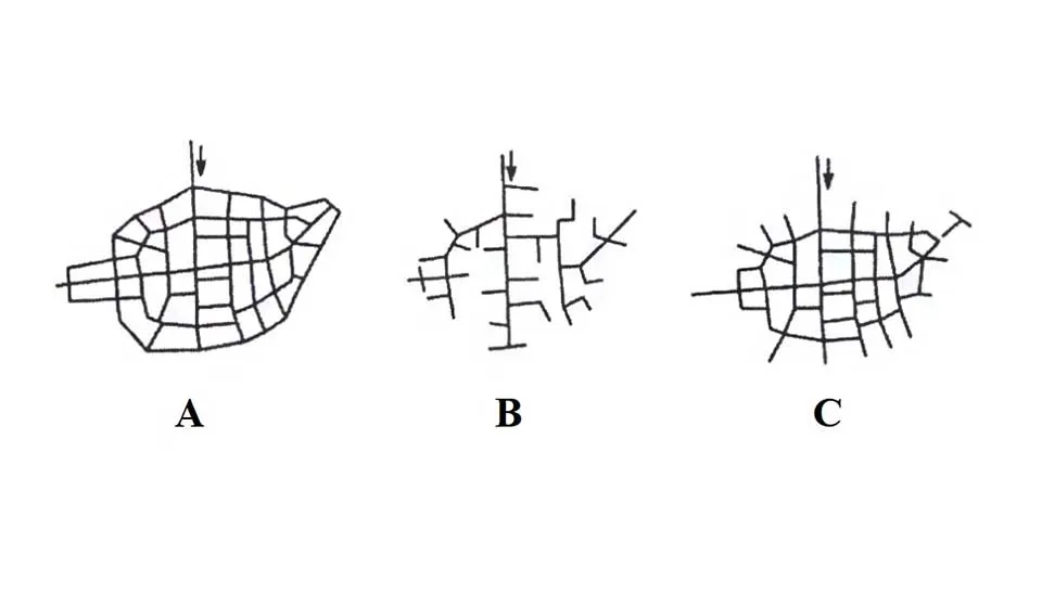
The design of water networks depends on the specific topography and the street layout in a given city. In the project, the mixed method will be used (Figure below).

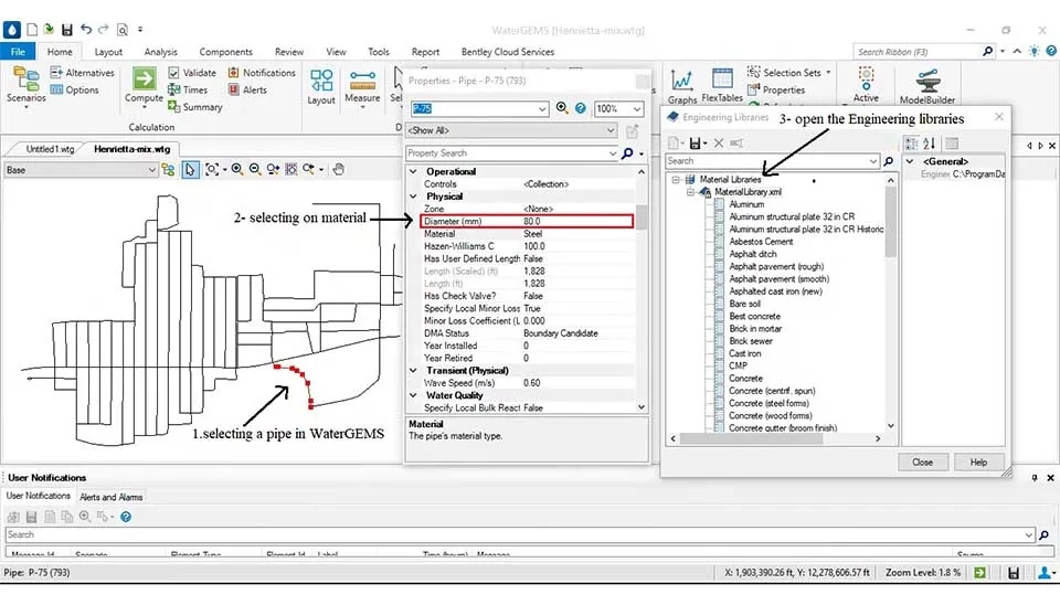
There is a material library in WaterGEMS Software for selecting the desired pipe, including various pipes such as steel, aluminum, asphalt ditch, concrete, etc. Hazen-Williams C is the main factor when choosing a pipe. This factor is different for any pipe. Additionally, there is no information about PE (Polyethylene); accordingly, it should be added manually to pipes; its method is as follows: First, select another pipe, for example, steel, then manually change the name to the pipe, as well as the relevant coefficients, such as Hazen-Williams C.

The figure below demonstrates changing a pipe to PE (polyethylene).

1. Selecting a pipe in WaterGEMS

2. Open the  properties and select the material

3.  Open the Engineering libraries to choose a pipe

4.10. Assigning Demands for Consumer 

There are several methods to assign demand between populations that  two methods use more, including:

1. Approximate methods 

2. Thiessen polygon

In the first method, demand is similarly divided between all nodes. Moreover, this method has a problem because the population is spread differently in the target city; instead, it is a suitable design method.

On the other hand, the Thiessen polygon is a suitable method for designing the water distribution network; the main advantage of this method is the allocation of demand among consumers in the same way. This method includes two allocation techniques: one based on density and another based on net area.

In a technique based on density and net area, it needs to have the net area of any house. However, this project does not access the net area of any home. Therefore, the approximate method is used to assign demands for consumers for the project. 

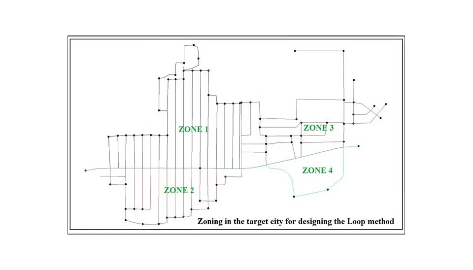
In this method, the demand is divided between specific nodes from pipes, including each pipe's beginning and end. The figure below illustrates how to divide demand between all nodes in this project.

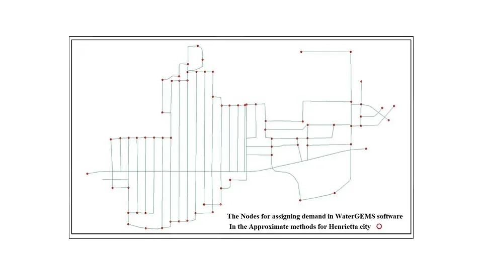
According to the upper figure, there are 76 nodes for assigning demand between them; therefore, all demand is divided into 76 nodes.

Q= 54.86 Gal/s , Node= 76 N ⇒ Q for every node ⇒ 29.32/76= 0.72 Gal/s (1.51 l/s)

4.11. The initial fundamentals of the water distribution system design 

It is crucial to observe some essential keys before designing:

1. The minimum and maximum diameter in distribution network pipes

For residential services, the diameter has to be between 0.5-0.8 inches (15-20 mm), and the distribution network's primary needs to be between 4-12 inches (100-300 mm). However, it may meet minimum or maximum velocity; you should choose a size bigger or smaller for these factors. 

2. The minimum and maximum velocity in distribution network pipes

It is essential to prevent sedimentation and ensure adequate flushing that the minimum velocity in pipes must be around one ft/s (0.3m/s), also avoiding excessive erosion and noise and prevent energy loss due to friction, the maximum velocity must be approximately 6.6-8.2 ft/s (2-2.5 m/s). In addition, the velocity selection in the design depends on the diameter of the pipe. This means that a pipe with a larger diameter is chosen for higher velocities.

3. The minimum and maximum velocity in pump charge and discharge pipe

The minimum and maximum velocities in pump suction and discharge pipe are crucial parameters that significantly impact the performance and efficiency of the pumping system. Additionally, the optimal size of the charge and discharge pipes directly impacts the prevention of pump cavitation. Additionally, the maximum size can be defined as the point at which the maximum velocity reaches approximately ten ft/s (3 m/s).

4. The minimum and maximum pressure at nodes

The minimum pressure is standard 20-30 psi (14-21 mH2o) at the consumer end; 20 psi (14 mH2o) is suitable for a house on one floor, and the pressure is suitable  30 psi (21 mH2o) for a house on two floors.

The maximum pressure is commonly 100-150 psi (70-105 mH2o) at the consumer end. It is necessary to select 70 psi (70 mH2o) because the sizing of pipes is going to be optimal unless there are different situations, such as different elevations between some nodes, where the system configuration of the distribution network can affect the pressure at nodes. The capacity and efficiency of pumps can affect the nodes' pressure. 

Note: One of the reasons engineers focus on selecting a pressure maximum of 100 psi (70 mH2O) is the water hammer, which creates pressures; hence, the water hammer is a threat to water transmission lines, and due to the increase of fluid working pressure, this phenomenon can be destructive to the water supply (Lema et al. 2016). Therefore, the water distribution network is designed for Henrietta City.

5. Results

To access these outputs, navigate to the Home tab in the WaterGEMS interface and left-click on the Flex Tables option. This action will open a dialog box that provides a comprehensive view of the system's data. Within this dialog, you can select specific components, such as pumps, pipes, or nodes, to display their corresponding data tables. These tables are organized to provide detailed information for each section, enabling engineers to analyze and interpret system performance efficiently.

5.1. Color Coding 

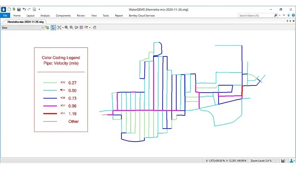
Color coding in WaterGEMS is a powerful visualization tool that allows engineers to represent hydraulic parameters such as velocity, pressure, and pipe diameter using a range of colors. This feature enhances the readability of complex water distribution networks, making critical variations or trends simple to identify. The Color Pipes By command allows you to select a pipe coloring scheme in your drawing. The coloring scheme chosen applies to all pipes in the drawing. Engineers can use this feature to show pipes with different velocities and diameters, and the nodes show based on different pressures.

The following sections will outline the steps to apply color coding in WaterGEMS.

1. Access the Element Symbology Manager:
   Go to View > Element Symbology.

2. Select the element type:
   Choose the element type you want to color code (e.g., pipes, maintenance holes, pumps).

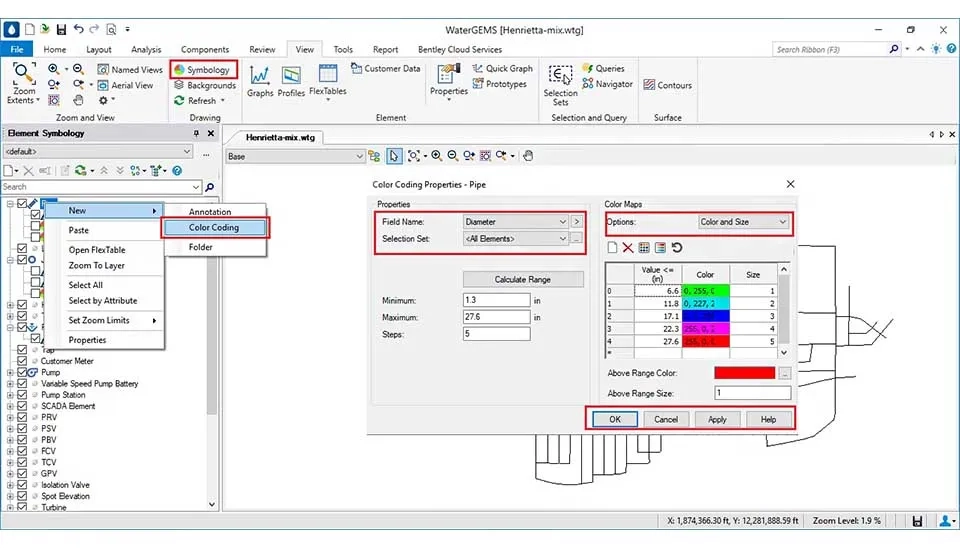
3. Create a New Color Coding:
   Right-click on the element type and select New > Color Coding.

4. Define Color Coding Properties:
   Field Name: Select the attribute you want to color code (e.g., flow velocity, pipe diameter, pressure).

Color Map Options: Choose whether to apply color, size, or both to represent the attribute values.

Color Map: Define the color range for the attribute values. You can use a predefined color palette or create a custom one.

Calculate Range: Automatically determine the minimum and maximum values for the attribute.

5. Apply Color Coding:

Color coding is a vital feature in WaterGEMS that enables the visualization and analysis of network elements, such as pipes and nodes, based on specific parameters like diameter, flow, or pressure. It provides an intuitive way to identify variations and patterns within the network. Once the color coding properties are defined, click Apply to implement the color coding to the selected elements, making the network easier to interpret and analyze.

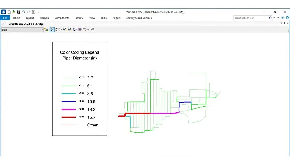
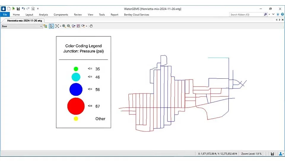
The figures below demonstrate the application of color coding for key parameters in the design of the Henrietta water distribution network. These include the diameter of pipes, the velocity within the pipes, and the pressure at nodes. Each parameter is visually represented using distinct color ranges, making it easier to identify variations, assess system performance, and pinpoint areas requiring attention. This approach ensures a comprehensive and clear analysis of the network's hydraulic behavior.

5.2. Pump

To meet the maximum water and pressure requirements of this project, it needs a pump with a flow rate of 29.32 Gal/s and a pressure of 433.5 feet, also, with 2900 RPM and a 220 butterfly diameter. This pump must be able to generate pressure between 20-70 psi. Finally, NPSH (Net Positive Suction Head) must be checked for this pump to prevent cavitation. The purpose of NPSH is to identify and avoid the operating conditions that lead to the vaporization of the fluid as it enters the pump – a condition known as flashing. In a centrifugal pump, the fluid’s pressure is at a minimum at the eye of the impeller. If the pressure here is below the vapor pressure of the fluid, bubbles are formed which pass on through the impeller vanes towards the discharge port. As the bubbles of vapor are transported into this higher-pressure region, they can spontaneously collapse in a damaging process called cavitation.

5.3. Pipes

The minimum pipe diameter is selected as 1.3 inches (32 mm), and a flow of velocity in this size is between 0.29-1.79 feet per second (0.08 - 0.59 m/s). Also, the maximum pipe diameter is selected as 15.7 inches (400 mm), and the velocity flow in this size is ذbetween 3.02 - 2.52  feet per second (0.92 - 0.76 m/s). 

The table below illustrates the results of diameter and velocity in the design for the city of Henrietta. The most important information from this table is the pipe length required for each diameter, as well as the demand and flow rates for each pipe. Therefore, the total pipe size needed for this project is 130,780 feet (39,862 meters). Additionally, the engineers can specify the length of each pipe size. For example, a pipe with a minimum diameter of 1.3 inches (30 mm) requires approximately 46,498 feet (14,172.6 meters), while a pipe with a diameter of 1.6 inches (40 mm) needs around 9,388 feet (2,841.5 meters); also, the maximum diameter is 15.7 inches (400 mm) with length 906 feet (23,012.4 meters). 

Download The Results of Pipes Required for Henrietta Case study

Due to the extensive amount of pipe output information, only ten rows are provided here to help engineers become familiar with the pertinent table.

The analysis of pipe P-1 in the project is shown in the first row of the table. The pipe is 940 feet long, 1.3 inches in diameter, and composed of steel. This pipe's water flow rate of 0.27 feet per second is comparatively low, indicating low flow intensity. The material and condition of the pipe are indicated by the Hazen-Williams coefficient (C), which is 100. The head loss gradient is 0.001 feet per foot and the flow rate is 0.69 gal/s, indicating a slight energy loss per foot of pipe as a result of friction. Given its relatively short length and low velocity, the calculated total head loss over the pipe length is 0.94 feet.

Similar analytic patterns are used in the following rows (P-2 to P-158), which assess the effectiveness and performance of each pipe in the system by concentrating on pipe-specific characteristics such as length, material, diameter, velocity, flow rate, and head loss values.

5.4. Nodes

The minimum and maximum pressure ranged from 24 to 67 psi (7.3 - 20.4 m). The table below provides information about all the nodes in the project. This table displays the output from the nodes, which typically includes essential information, such as pressure and demand for each node in water supply systems. This information helps engineers understand how pipe thickness is calculated for each size. 

Several methods are available for calculating the required wall thickness of a piping system by ASME B31.3. This formula helps determine the minimum required wall thickness of a pipe based on its internal pressure, diameter, and material properties.

Due to the extensive amount of output information regarding nodes, only ten rows are provided here to help engineers become familiar with the pertinent table.

Click To Download Final Outputof Required Pipes and Nodes for Designing Network Distribution in Henrietta .

The initial row of the table presents an examination of node J-01 inside the project. The altitude of this node is 931.03 ft, and its demand is 0.4 gal/s, signifying the water necessity at this site. The hydraulic grade is 1008.92 ft, indicating the energy level of the water at this node, which encompasses both elevation and pressure head. The pressure at this node is 34 psi, signifying the force applied by the water on the system at this location. 

The remaining rows (J-02 to J-111) follow a similar analysis pattern, examining elevation, demand, hydraulic grade, and pressure for each node. This approach ensures that the water distribution system meets the hydraulic requirements at all nodes, maintaining adequate pressure and flow rates throughout the network.

6. Conclusion

As a consequence, the WaterGEMS software is specific hydraulic software with advanced capabilities for analyzing and designing water distribution networks, including collaboration, building geographic models, optimization, and management. The advantages of WaterGEMS software are:

• It is a friendly and easy-to-use interface.

• Support for steady state and long-term simulations.

• Ability to analyze water quality and identify pressure zones.

The essential requirements for designing the water distribution networks include predicting the population for 30 years into the future and calculating demand based on peak factors hourly and daily.  It is also crucial to choose and define reservoirs and pumps for simulation. Finally, this software can present suitable pipes for any demand and pressure.

The water distribution network was designed based on a population of 3900 people and a demand of 29.32 Gal/s for Henrietta. The method that is mixed with branched and looped is chosen to design the distribution network. Also, it needs a pump with a demand of 29.32Gal/s, a pressure of 433.5 feet, 2900 RPM, and a 220 butterfly diameter. The steel pipe is calculated with a length of 130710 feet by WaterGEMS software. Diameters minimum and maximum are included from 1.3 feet to 27.6 feet. Besides, the optimal pressure for this project is designed to be between  30 and 69 psi.